Week 6: Additional Information: Bayesian Revision, EVSI & Utility
This week’s big question: tests and surveys can be wrong. How should an imperfect signal change your beliefs, and how much is that signal worth paying for?
Before the week
Read: Taylor, Introduction to Management Science (13e), Chapter 12, pp. 596–604, and start with Chapter 11, pp. 550–551, the short Bayesian analysis section. The chapter PDFs are in Canvas Files.
| Pages | Section | This week |
|---|---|---|
| 596–600 | Decision Analysis with Additional Information | Read. Bayes’ rule on the investor’s tree: a prior becomes a posterior |
| 600–601 | Computing Posterior Probabilities with Tables | Read. The five-column table Monday builds by hand |
| 601–602 | Computing Posterior Probabilities with Excel | Skim. The optional Bayes calculator checks your hand work |
| 602 | The Expected Value of Sample Information | Read. Wednesday’s core skill, plus efficiency |
| 602–604 | Utility | Read. Utiles, risk averters, risk takers; the curve itself is ours |
Stop where the Summary begins on p. 604. The top of p. 596 finishes an Excel QM walk-through of sequential trees; skip straight to the “Additional Information” heading.
Then the warm-up self-check, on conditional probability and what a “prior” means:
Session 1: Mon, Sep 28 · Bayesian revision: prior → posterior
🧩 Puzzle
The developer. A developer is deciding whether to invest in a project. If demand turns out High the project is worth +\$200k; if demand is Low it loses −\$100k. Right now their belief is High 0.6, Low 0.4. Before committing, they could buy a market survey, but a survey only ever comes back “favorable” or “unfavorable,” and it isn’t perfect. How should a survey result actually change what they believe about demand?
Without a survey, investing has expected value \(0.6(200) + 0.4(-100) = 80\), so invest. The survey is not about the 80. It is about whether the 0.6 should still be 0.6 once the survey has spoken.
Build the skill 1: likelihoods: how reliable is the signal?
A survey is described by its track record, written as conditional probabilities \(P(\text{result} \mid \text{state})\), the likelihoods. When demand is truly High this survey calls “Favorable” 95% of the time; when demand is truly Low it still says “Favorable” 45% of the time, the false alarm. Laid out as a table, one row per state:
| If demand is truly | Says Favorable | Says Unfavorable | Row sum |
|---|---|---|---|
| High | 0.95 | 0.05 | 1.00 |
| Low | 0.45 | 0.55 | 1.00 |
Each row runs “state → result” and sums to 1, because the survey must say something. A vendor’s headline “95% accurate” is only the top-left cell; the 0.45 is a Low market that still reads Favorable, almost half of the time. But on survey day you hold the result and want the state: “result → state.” Flipping that direction is what the rest of the session does, first by counting and then with Bayes’ rule.
The flip, counted on 1,000 projects
Run the survey on 1,000 projects like the developer’s and you can count your way to the flip. The prior splits them 600 High and 400 Low. Inside each group the track record says how the survey reads: Favorable on \(0.95 \times 600 = 570\) of the High projects and on \(0.45 \times 400 = 180\) of the Low ones; the other 30 High and 220 Low read Unfavorable.
Now the survey says Favorable. What should the 0.6 become?
- Two joints. 570 of the 1,000 are High and Favorable, \(0.6 \times 0.95 = 0.57\); 180 are Low and Favorable, \(0.4 \times 0.45 = 0.18\).
- Their sum, the marginal. Favorable on \(570 + 180 = 750\) of the 1,000, \(0.57 + 0.18 = 0.75\): the chance the survey comes back Favorable at all, before you have seen it.
- The ratio, the posterior. Those 750 Favorable reads are the new whole, and 570 of them are High: \(570 / 750 = 0.57 / 0.75 = \mathbf{0.76}\).
The survey moves 0.6 to 0.76. Two joints, their sum, then the ratio; the \$200k and the \$100k never entered it. That is the whole move this week: a result you can see (a survey read) revises a belief about a state you cannot (true demand).
Read the same 1,000 the other way and it is where a track record comes from. A vendor who has run this survey on 600 High markets and watched it read Favorable on 570 of them reports \(570 / 600 = 0.95\); the 0.45 is 180 of the 400 Low ones. Each likelihood divides by its own row’s total, never by the 1,000. The take-home hands you counts like these and asks for the likelihoods, so choosing the denominator is the modelling step there.
Build the skill 2: Bayes’ rule: joint, then posterior
Four words carry the count, and every table this week climbs them in order: prior, likelihood, joint, posterior. (Taylor’s Table 12.12 heads the same columns prior, conditional, prior × conditional and posterior, and Chapter 11 calls the prior a marginal and the product a joint probability; likelihood is our word for the conditional.)
- Prior: what you believed before the signal. High 0.6, the 600 of 1,000.
- Likelihood: how the signal behaves given the truth. \(P(\text{Fav} \mid \text{High}) = 0.95\).
- Joint: prior × likelihood, both true at once. \(0.6 \times 0.95 = 0.57\).
- Posterior: what you believe after the signal, the joint re-based on its column. 0.76.
Bayes’ rule writes that ratio in probabilities: build the joint probability of a state and result, then divide by the probability of the observed result:
\(P(\text{state} \mid \text{result}) = \dfrac{P(\text{result} \mid \text{state})\,P(\text{state})}{P(\text{result})}\).
On top, the joint: likelihood times prior, \(0.95 \times 0.6 = 0.57\). Underneath, the marginal: every joint for that result, added down the column, \(0.57 + 0.18 = 0.75\). The ratio is the posterior, the same cases re-based on the world where the survey said Favorable, \(0.57 / 0.75 = 0.76\). Because the denominator is the column sum, the posteriors in each column must add to 1, a built-in check you should run every time.
The widget below draws that same count. Its top bar is the 1,000 projects split by the prior; the second splits the same 1,000 by what the survey reads, solid for Favorable and pale for Unfavorable. Press Favorable survey: the Unfavorable reads fade, the 570 + 180 = 750 Favorable reads are kept, and the bottom bar re-bases them to a whole, 570 of 750, the posterior 0.76. Press Unfavorable survey for 30 of 250, 0.12, and Back to prior to start again. The slider moves the prior, which Build the skill 3 needs:
Now work both columns by hand so the machine is never a black box. Taylor lays this out as a five-column table (his Table 12.12): state, prior, conditional (likelihood), joint, posterior. He works the positive report and says the negative one is “computed similarly”; the table below puts both report outcomes side by side. Favorable lifted High to 0.76; before you read the right half, guess whether Unfavorable pulls it below 0.5:
| State | Prior | \(P(\text{Fav}\mid\text{state})\) | Joint (Fav) | Posterior \(\mid\) Fav | \(P(\text{Unfav}\mid\text{state})\) | Joint (Unfav) | Posterior \(\mid\) Unfav |
|---|---|---|---|---|---|---|---|
| High | 0.6 | 0.95 | 0.57 | 0.76 | 0.05 | 0.03 | 0.12 |
| Low | 0.4 | 0.45 | 0.18 | 0.24 | 0.55 | 0.22 | 0.88 |
| Σ | 0.75 | 1.00 | 0.25 | 1.00 |
Read the bottom row twice. The joint column sums are the marginals \(P(\text{Favorable}) = 0.75\) and \(P(\text{Unfavorable}) = 0.25\), and they themselves add to 1, because the survey must return some result. The posterior columns each sum to 1, confirming you renormalized correctly. So a Favorable survey lifts your belief in High demand from 0.6 → 0.76, and an Unfavorable survey flips you the other way to High 0.12 / Low 0.88. Those four posteriors are the inputs to everything in Session 2.
Keep the denominators in view: the likelihood \(0.95 = 570/600\) is a share of High projects, while the posterior \(0.76 = 570/750\) is a share of Favorable reads. The prior, 0.60, describes demand; the report marginal, 0.75, describes what the survey says. Each number answers a different question.
Build the skill 3: the base rate: the same survey on a long-shot project
The developer’s 0.6 was close to even. They are also weighing a second project, on a parcel at the edge of town, where they put High demand at only 0.1. Same survey, same track record (Favorable on 95% of High markets and on 45% of Low ones), so count it on 1,000 projects like this one: 100 High and 900 Low. The survey reads Favorable on \(0.95 \times 100 = 95\) of the High projects and on \(0.45 \times 900 = 405\) of the Low ones, 500 in all. A Favorable read arrives:
| State | Prior | \(P(\text{Fav}\mid\text{state})\) | Joint (Fav) | Posterior \(\mid\) Fav |
|---|---|---|---|---|
| High | 0.1 | 0.95 | 0.095 | 0.19 |
| Low | 0.9 | 0.45 | 0.405 | 0.81 |
| Σ | 0.50 | 1.00 |
The Favorable read that took the first project from 0.6 to 0.76 takes this one from 0.1 to only \(0.095 / 0.50 = 0.19\). About four Favorable reads in five come from Low projects, 405 of the 500, because Low projects are nine times as common: a 45% false-alarm rate on 900 of them outnumbers a 95% hit rate on 100. The track record did not change; the prior did. That prior is the base rate. Headline accuracy is a likelihood, the number you act on is the posterior, and the base rate sits between them. Watch it in the widget above: drag its prior down to 0.10 and press Favorable survey, and the kept reads are 95 High against 405 Low, re-based to 0.19. Wednesday asks what a survey is worth on a long shot like this one.
Bayesian revision with software
The optional Bayes calculator starts with this developer’s survey. Choose Favorable or Unfavorable to see the prior, likelihood, joint, and posterior, with the marginal and the arithmetic below the table. Change the prior to 0.1 to check the long-shot project, or enter your own labels and probabilities. It handles two states and two signal outcomes, with nothing to install.
Use it to check a revision you have already done by hand. The take-home asks you to produce the posterior yourself, and so can an exam. For the payoff decisions in Session 2, keep using the decision tree builder.
In practice: the inputs are estimates, and they come from different places
- Priors are often subjective; likelihoods are often a track record. Chapter 11 separates classical, relative-frequency, and subjective probability. A prior like “High 0.6” is usually a subjective read of the market, and “different people will often arrive at different subjective probabilities,” so two analysts can start from different priors and reach different posteriors from the same survey. A likelihood like \(P(\text{Favorable} \mid \text{High}) = 0.95\) is usually a relative-frequency number: the vendor’s hit rate across past jobs.
- Vendors quote their best case. That 0.95 is the flattering number. Treat it like any other input. Ask how it was measured, and re-run the table with a less generous value to see if your decision flips.
- Base rates matter. The same survey that lifts the first project to 0.76 lifts the long-shot project only to 0.19. This is the famous reason a positive rare-disease test can still be probably wrong. Always carry the prior through the math instead of trusting the headline accuracy.
Back to the puzzle
The developer doesn’t have to treat the survey as gospel or ignore it. Bayes’ rule converts “High 0.6 / Low 0.4” plus a survey result into a revised belief: Favorable → High 0.76 / Low 0.24, Unfavorable → High 0.12 / Low 0.88. Before either result arrives, Favorable is the likelier one: \(0.75\) against \(0.25\), and those two marginals are what Wednesday’s tree hangs on its first circle. How far a result can move you depends on where you start: on the long-shot project the same Favorable read lifts 0.1 only to 0.19. Revised beliefs are a means, not an answer. Given the revision, is the survey worth its price?
In-class group practice (wrap-up)
To close Session 1, run one Bayesian revision by hand in your group.
Write every member’s name on the sheet. You have 15 minutes for the practice, then two minutes to photograph your group’s own attempt before the solutions are shown. One member uploads the photo to Canvas by the end of class; participation credit is for attempting the work.
The instructor uses the final eight minutes to demonstrate the handout’s method, check the main results with units, and explain a common mistake. This demonstration closes the session.
- Download: Week 6 group practice (Word)
Session 2: Wed, Sep 30 · EVSI, efficiency & utility
🧩 Puzzle
The developer can invest now, or buy a survey and decide after seeing its result. How much more could they earn, on average, by using the survey? What is the most they should pay for it? And separately: the project risks a real \$100k loss. Even if the expected value says “invest,” why might a cautious owner still walk away?
Build the skill 1: the survey-or-not tree, and EVSI
The developer earns +\$200k if demand is High and loses \$100k if it is Low. Not investing pays \$0. All figures below are in thousands of dollars, so 200 means \$200,000.
The survey can help because you get to choose after hearing its result: invest if the revised outlook is good enough, or stay out if it is not. The expected value of sample information (EVSI) measures how much that opportunity improves your expected payoff, before subtracting the survey’s fee. Here, “sample information” means the imperfect information supplied by the survey.
To find that improvement, compare two plans: choose without a survey, or get the survey and choose after each possible report. Leave the fee off while valuing those plans; their difference will tell you the most you should pay. You must average over both reports because you do not know which one will arrive.
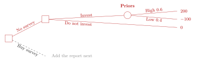
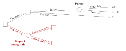
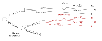
Build the tree from left to right, in the order things happen: choose whether to get the survey, hear its report if you do, choose whether to invest, then learn the demand. A square marks a choice you control; a circle marks an uncertain event. Each picture keeps the previous branches in place. Red marks the components you add in that step. On a narrow screen, scroll across a picture to read its labels.
Step 1: draw the choice without a survey
Start with a square for No survey / Buy survey. Along No survey, add another square for Invest / Do not invest. Invest leads to a demand circle with High and Low branches; Do not invest ends at 0. With no new information, put the priors, 0.6 and 0.4, on the demand branches. Put 200 and −100 at their ends.
Step 2: add the reports you might receive
Along Buy survey, draw a circle because you cannot choose the report. Its two branches are Favorable and Unfavorable. Use Monday’s marginals: Favorable \(0.57 + 0.18 = 0.75\); Unfavorable \(0.03 + 0.22 = 0.25\). These describe how often each report arrives, before you have seen it. Put a new decision square at the end of each report branch: you still get to choose whether to invest.
Step 3: build the choice after Favorable
From the Favorable square, add Invest and Do not invest again. Invest leads to another demand circle. You now know the report was Favorable, so use the posteriors: High \(0.57/0.75 = 0.76\) and Low \(0.18/0.75 = 0.24\). Those probabilities go on the demand branches under Favorable. The report changes your beliefs; the payoffs are still 200, −100, and 0.
Step 4: build the choice after Unfavorable
Repeat those two choices at the Unfavorable square. Its demand circle uses that report’s posteriors: High \(0.03/0.25 = 0.12\) and Low \(0.22/0.25 = 0.88\). Keep the same three payoffs. Do not prune a choice yet; build all the options before deciding which is best.
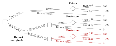
Check each circle on its own: \(0.6+0.4=1\) without a survey, \(0.75+0.25=1\) for the reports, \(0.76+0.24=1\) after Favorable, and \(0.12+0.88=1\) after Unfavorable.
The report circle carries the marginals; the demand circles under each report carry the posteriors. The No survey demand circle keeps the priors. The likelihoods from the vendor’s track record helped you calculate these probabilities; they do not replace them on this tree.
Now fold the completed tree
Work from right to left: average at circles, keep the better branch at squares. In the completed tree below, press Fold back to reveal the values one layer at a time; Reset hides them again.
The fold makes three investment decisions. At each square, compare investing with staying out at 0:
| Information available | Expected payoff if you invest | Best choice | Value kept at the square |
|---|---|---|---|
| No survey | \(0.6(200)+0.4(-100)=80\) | Invest | 80 |
| Favorable report | \(0.76(200)+0.24(-100)=128\) | Invest | 128 |
| Unfavorable report | \(0.12(200)+0.88(-100)=-64\) | Do not invest | 0 |
Without the survey, the best plan is to invest, worth 80. With the survey, the plan is to invest after Favorable and stay out after Unfavorable. Before you receive a report, Favorable has probability 0.75 and Unfavorable has probability 0.25. Average the values of the choices you will make:
\[0.75(128)+0.25(0)=96.\]The 96 is the expected payoff from following the survey-based plan, before paying for the survey. It includes the investment earnings. The survey itself is worth only the improvement over the 80 you could earn without it.
EVSI: the improvement before the survey fee
Subtract the best expected payoff without the survey from the expected payoff with it:
\(\text{EVSI}=96-80=16\quad\text{(\$ thousands)}\).
Using the survey improves expected payoff by \$16k. That is the most you could pay without making the survey-based plan worse than investing without it. It is an expected improvement, not a guaranteed profit on this one project.
Now consider the fee. Suppose the survey costs \$10k. The survey-based plan then has expected payoff \(96-10=86\), compared with 80 without it. Its net advantage is \(86-80=6\), or \$6k. Equivalently, subtract the fee from EVSI: \(16-10=6\). Subtract the fee only once.
| Survey fee | Decision if you maximize expected dollars |
|---|---|
| Below \$16k | Buy it: the expected improvement exceeds the fee. |
| Exactly \$16k | Either plan: both have the same expected payoff. |
| Above \$16k | Skip it: the fee exceeds the expected improvement. |
Why the survey adds value, and when it adds none
The survey adds value because Unfavorable changes the action. Without a survey you would invest. After Unfavorable, investing has expected payoff −64, so you stay out at 0 instead. That report arrives with probability 0.25, giving an expected improvement of \(0.25[0-(-64)]=16\). After Favorable, you still invest, so the action does not change. This explains the same \$16k found by subtracting the two plans.
For a contrast, keep the developer’s payoffs and survey but set the prior probability of High demand to 0.1, as on the long-shot project. The posteriors are High 0.19 after Favorable and 0.01 after Unfavorable:
| Information available | Expected payoff if you invest | Best choice |
|---|---|---|
| No survey | \(0.1(200)+0.9(-100)=-70\) | Stay out: 0 |
| Favorable report | \(0.19(200)+0.81(-100)=-43\) | Stay out: 0 |
| Unfavorable report | \(0.01(200)+0.99(-100)=-97\) | Stay out: 0 |
Neither report changes the choice. Both plans are worth 0 before the fee, so EVSI is 0. A survey can change your beliefs without improving your decision.
Compare the survey with perfect information
EVSI prices this particular survey. EVPI gives an upper bound: the improvement you could get from knowing demand perfectly before deciding. A perfect forecast lets the developer invest when demand is High and stay out when it is Low:
\[0.6(200)+0.4(0)=120.\]That plan is worth 120 before the forecast’s fee. Compared with the same no-survey baseline of 80, EVPI is \(120-80=40\), or \$40k. The survey’s efficiency compares its improvement with this perfect-information improvement:
\(\text{efficiency}=\frac{\text{EVSI}}{\text{EVPI}}=\frac{16}{40}=\mathbf{40\%}\).
This survey captures 40% of the value of perfect information, useful to know before paying for it. Its track record is what makes it noisy: it misses a High market one time in twenty (\(P(\text{Unfavorable} \mid \text{High}) = 0.05\)) and reads a Low one as Favorable almost half of the time (\(P(\text{Favorable} \mid \text{Low}) = 0.45\)). Of the \$24k the survey leaves on the table, the misses cost \$6k and the false alarms \$18k. A miss happens 3% of the time (\(0.6 \times 0.05\)) and forfeits the \$200k upside; a false alarm happens 18% of the time (\(0.4 \times 0.45\)) and walks you into the \$100k loss. And notice EVSI (\$16k) \(\le\) EVPI (\$40k): an imperfect signal can never be worth more than perfect information. Equality is possible if the signal lets you choose as well as perfect information would.
A different survey, a different EVSI
To see how a different track record changes the value, keep the developer, the payoffs, the prior, and the \$40k ceiling, and change only the track record: a sharper survey with \(P(\text{Fav} \mid \text{High}) = 0.9\) and \(P(\text{Fav} \mid \text{Low}) = 0.1\). After Favorable the joints are \(0.54\) and \(0.04\), the marginal \(0.58\), and the posterior \(0.54 / 0.58 \approx \mathbf{0.93}\); investing is worth \(0.93(200) + 0.07(-100) \approx 179\), so the developer invests. After Unfavorable (joints \(0.06\) and \(0.36\), marginal \(0.42\), posterior High \(\approx 0.14\)) investing is worth about \(-57\), so the developer backs out and keeps 0. The survey branch is \(0.58 \times 179 \approx 104\) (exactly \(0.54(200) - 0.04(100) = 104\)) against 80 blind, so EVSI \(= 104 - 80 = \mathbf{24}\) against the same EVPI of 40: an efficiency of 60%. Two reference points now anchor the 0%-to-100% scale, on one tree: the original survey at 40% and a sharper one at 60%. The payoffs and the prior are the developer’s; the track record is the difference. The sharper survey misses more High markets (10% instead of 5%), but cuts false alarms from 45% to 10%. On these payoffs, that trade raises its value.
The same tree is an example in the course’s tree builder: File, then Week 6: the developer’s survey. Its posteriors are written from the prior and the track record by Bayes’ rule, so in its What if tab, setting favIfHigh to 0.9 and favIfLow to 0.1 turns it into the sharper survey, whose branch folds to 104, and sweeping price shows the survey stop paying at 16, its EVSI.
Why EVPI is also the lowest expected regret. There is a second, intuitive route to that \$40k ceiling. Taylor notes that the EV criterion and the expected-opportunity-loss criterion always pick the same decision, and that EVPI equals the expected opportunity loss (EOL) of the best decision, the expected regret you cannot avoid even when you choose well. Here the best no-info act (Invest) regrets 0 if demand is High and \$100k if it is Low (you should have stayed out), so its EOL is \(0.4(100) = 40\): \$40k of unavoidable expected regret, which is exactly EVPI. So whether you think of it as “the value of a crystal ball” or “the regret you’re stuck with,” the ceiling that bounds EVSI is the same number.
Build the skill 2: utility & risk attitudes
Set the survey aside and look at the gamble underneath it. Expected value says invest: \$80k, done. Yet a real owner staring at a possible \$100k loss might still decline. They’re not bad at arithmetic, they value outcomes nonlinearly. That’s the idea of utility: instead of maximizing expected dollars, you maximize expected utility, where utility \(u(x)\) captures how much each dollar amount is actually worth to you.
- Risk-averse: utility curve is concave (bends down). The pain of losing \$100k outweighs the joy of gaining \$100k, so you’ll skip some positive-EV gambles. Most people and firms are risk-averse for big stakes.
- Risk-neutral: utility is a straight line; maximizing expected utility is identical to maximizing expected dollars.
- Risk-seeking: utility curve is convex (bends up); you’ll accept fair or even unfavorable gambles for the chance at the upside (think lottery tickets).
(Taylor’s own text calls these risk averters and risk takers, with the linear case “indifferent to risk”. The same three attitudes under older names.) Utility replaces each dollar amount with what it is worth to you, then re-folds. The rules are unchanged; the payoffs are not.
Make it bite. Cover for the \$100k loss. A partner offers to absorb the developer’s \$100k loss if demand comes in Low, for a fee of \$50k paid up front whatever happens. The expected loss avoided is \(0.4 \times 100 = \mathbf{40}\), less than the 50 it costs. Covered, investing is worth \(0.6(200 - 50) + 0.4(-100 + 100 - 50) = 0.6(150) + 0.4(-50) = \mathbf{70}\) against 80 bare, so the cover costs 10 in expectation, which is \(50 - 40\). Pure EV says skip it. A cautious owner buys it anyway, because a single \$100k loss could end the firm. Taylor’s auto-insurance example (Table 12.13) makes the same point: the policy costs more than the expected loss, and people buy it. EV says no, a risk-averse human says yes. Buying insurance is the everyday proof that people maximize utility, not dollars.
Certainty equivalent: the guaranteed payment that matches the gamble
Imagine the developer can exchange the project for a guaranteed payment. The project still has two possible outcomes: a 60% chance of gaining \$200k and a 40% chance of losing \$100k. Ask the owner:
What guaranteed payment would make you equally willing to take that payment or keep the project?
That amount is the certainty equivalent (CE). “Equally willing” means the owner has no preference between the two options. For the owner represented by the widget’s Risk-averse curve, it is about \$28k:
| Take the project | Take the guaranteed payment |
|---|---|
| Gain \$200k with probability 0.6; lose \$100k with probability 0.4 | Receive about \$28k for certain |
| Uncertain outcome | No uncertainty |
This owner values these two options equally. Offer more than \$28k for certain and they prefer the payment; offer less and they prefer the project. The project still has expected value \(0.6(200)+0.4(-100)=80\), or \$80k. Its CE is lower because this owner is willing to give up some expected dollars to avoid the possible loss.
CE depends on the owner’s preferences. You can find it by asking the comparison question above, or read it from a utility curve that represents those preferences. The payoffs and probabilities determine EV; they do not determine CE by themselves. The \$28k here comes from the illustrative curve, not from a rule that all risk-averse people must use.
Read the certainty equivalent from the utility curve
A utility curve converts a guaranteed dollar amount into how much the owner values it. To find CE, use that curve in reverse: find the guaranteed amount that has the same utility as the gamble.
- Value the two outcomes in utiles. On this curve, the worst outcome, −\$100k, has utility 0 and the best, +\$200k, has utility 1.
- Average those utilities using the probabilities. The gamble’s expected utility is \(0.6(1)+0.4(0)=0.60\) utiles.
- Find the guaranteed amount with utility 0.60. Start at 0.60 on the vertical axis, move across to the curve, and then down to the dollar axis. On the Risk-averse curve, you reach about \$28k.
For this gamble, match its expected utility of 0.60:
\[u(\text{CE})=0.60.\]Here, \(u(\$28k)\approx0.60\), so a sure \$28k and the gamble have the same value to this owner. 0.60 is a utility value; \$28k is the certainty equivalent in money.
Risk premium: how much expected payoff the owner would give up
Once you know CE, compare it with EV. The risk premium is EV minus CE:
\[\text{risk premium}=80-28=52.\]In thousands of dollars, this owner is willing to give up about \$52k of expected payoff to replace the risky project with a guaranteed \$28k. The risk premium measures that trade; it is not a bill they must pay. For this risk-averse owner CE is below EV; a risk-neutral owner has CE equal to EV, and a risk-seeking owner can have CE above EV.
Beyond the book. Taylor introduces utility with utiles and risk attitudes. The curve, certainty equivalent, and risk premium extend that treatment so you can compare a gamble with a guaranteed payment.
The widget uses the developer’s payoffs in thousands of dollars. Press Risk-averse and trace the 0.60 utility level to CE 28 on the curve. Press Risk-neutral: the same gamble now has CE 80. Press Risk-seeking: CE rises to about 122. The payoffs and probabilities stay fixed; only preferences change. The hollow dot marks not investing, a sure \$0, which is a separate available choice. Its dashed vertical line connects the dot to 0 on the payoff axis. For the Risk-averse preset, 0 is below CE 28, so this owner still prefers investing to staying out:
A more cautious owner can prefer not to invest
A CE of \$28k does not mean the owner rejects the project: the actual alternative, staying out, pays only \$0. Now consider a more cautious owner, who puts a higher value on avoiding the loss. Keep the same payoffs and probabilities but use this utility scale:
| Payoff (thousands of dollars) | Utility |
|---|---|
| −100 | 0 |
| 0 | 0.65 |
| 200 | 1 |
Re-fold the no-survey choice in utiles. Investing has expected utility \(0.6(1)+0.4(0)=0.60\); staying out has utility \(u(0)=0.65\). This owner stays out because 0.65 exceeds 0.60. Their CE must be below \$0: even a sure \$0 is worth more to them than the gamble.
To calculate CE from the table, assume a straight line between the listed utility points. The target, 0.60 utiles, lies between 0 and 0.65, so use the payoff interval from −100 to 0. Move the fraction \(0.60/0.65\) of the way across that interval:
\[\text{CE}=-100+\frac{0.60}{0.65}(100)\approx-7.7.\]This is about −\$8k. A negative CE means this owner is indifferent between the project and a small sure loss. Staying out at \$0 is better than either. The risk premium is about \(80-(-7.7)=87.7\), or \$88k. This is the same CE calculation as before: match the gamble’s utility with the utility of a guaranteed amount, then read that amount in dollars.
The tree builder has this comparison as Week 6: the developer in utiles. Its What if tab sweeps u0, the utility of \$0; staying out wins once u0 exceeds the gamble’s 0.60. In the widget above, drag toward more cautious until the hollow dot for a sure \$0 is above 0.60. The owner then walks away. The widget uses smooth curves, so its exact CE can differ from the straight-line calculation above; a CE below 0 gives the same decision in either case.
In practice: neither perfect information nor perfect rationality exists
- Imperfect is the normal case. “Perfect information” almost never exists. Surveys, tests, and pilots are all imperfect. Here EVSI is \$16k, below the \$40k EVPI. The efficiency ratio tells you how much of the ideal a real study buys you, so you don’t overpay (40% here; 60% for the sharper survey).
- The revision is only as good as its inputs. The posteriors rest on estimated priors and estimated likelihoods. If either is off, EVSI is off. Re-run it with pessimistic likelihoods before trusting it.
- People are not EV-maximizers. Loss aversion, limited capital, and “bet-the-company” stakes mean a positive-EV decision can still be the wrong human decision. Utility doesn’t excuse the math: it extends it, by letting you re-fold the tree in utiles instead of dollars. Report the dollar answer and the utility answer, and say which scale the recommendation is on.
Back to the puzzle
The best plan without a survey is worth \$80k. Getting the survey and acting on its reports raises expected payoff to \$96k before its fee. The improvement is \$16k, the EVSI. Buy the survey if its fee is below that amount; at exactly \$16k, the plans tie. This survey captures 40% of the \$40k a perfect forecast would be worth. That \$40k is also the unavoidable expected regret of investing blind, the same ceiling seen from the opportunity-loss side. On the long-shot project the same survey is worth nothing, because no report would change the decision. And the cautious owner who passes on a +\$80k gamble isn’t being irrational: a concave utility curve tells you which guaranteed amount they value as much as the gamble. The widget’s risk-averse owner is indifferent between the project and a sure \$28k, and still invests rather than stay out at \$0. The more cautious owner’s CE is below \$0, so that owner prefers not to invest. Decision analysis gives you both the dollar value of information and the language to respect risk attitude.
After-class check
A few questions spanning the whole week: Bayesian revision, posteriors, EVSI vs. EVPI, efficiency, and risk attitudes. Retry as many times as you like; nothing is submitted.
Weekly take-home (graded: submit on Canvas)
This week’s take-home is a Bayesian revision, EVSI and utility model for a state workforce agency deciding whether to fund a job-training program, plus one picture of your tree. The likelihoods are not given to you: the case brief reports an evaluator’s validation study as raw counts, and the prior comes from a different source altogether: the agency’s own portfolio. In the Your model block you say which number is the prior and write both conditional probabilities out in words, because confusing them is the error this week exists to fix. Then you revise and price the assessment against its own ceiling. Build the assessment-or-not tree in the tree builder as you go, with your marginals on the read circle, your posteriors on the circles after each read and the assessment’s price left off, press Fold back, and check it against your workbook. File, then Download a picture (PNG), saves the picture you submit; a screenshot of the whole folded tree works too. Finally you re-fold the whole decision on the director’s utility scale, where the recommendation changes. Two short responses plus the required AI-use disclosure go on the Free responses sheet. Upload two files on Canvas: the completed .xlsx and the picture of your folded tree.