Week 7: Linear Programming: Formulation & Graphical Solution
This week’s big question: when resources are limited, exactly how much of each product should you make to earn the most? You will learn to turn that question into a linear program and solve it by hand, the foundation for everything in Weeks 8–11.
Before the week
Read: Taylor, Introduction to Management Science (13e), Chapter 2, pp. 54–80. Twenty-seven pages, and this is the one chapter all term whose whole body is on target, so read it straight through. The chapter PDF is in Canvas Files.
| Pages | Section | This week |
|---|---|---|
| 54–58 | Model Formulation; A Maximization Model Example | Read. Monday: decision variables, objective, constraints |
| 58–70 | Graphical Solutions of Linear Programming Models | Read. Wednesday: the feasible region, the corners, and slack variables (p. 67) |
| 70–76 | A Minimization Model Example | Read. Wednesday’s second half: ≥ requirements and surplus variables (p. 75) |
| 76–79 | Irregular Types of Linear Programming Problems | Read. Multiple optima, an infeasible problem, an unbounded problem |
| 79–80 | Characteristics of Linear Programming Problems | Read. The four assumptions, in the book’s own words |
Stop where the Summary begins on p. 80. This is also the only chapter with no QM for Windows or Excel QM section, which is why nothing in it is skipped.
Then the warm-up self-check: the one prerequisite the graph method needs (plotting lines and inequalities), plus a quick check on what makes an objective legal:
Session 1: Mon, Oct 5 · Formulating a linear program
🧩 Puzzle
The corner bakery. Each morning you bake croissant batches and muffin batches. A croissant batch earns \$4 profit; a muffin batch \$3. But you are limited: the oven gives you 10 hours (2 h per croissant batch, 1 h per muffin batch), and you have 15 units of flour (1 per croissant batch, 3 per muffin batch). How many batches of each should you bake to make the most profit?
You cannot reliably eyeball this, and guessing wastes money. By the end of this session you will be able to write it as a model that can be solved exactly.
This little bakery is a toy stand-in for a serious idea. Linear programming (LP) is the workhorse behind production planning in factories, diet and feed blending on farms, fuel mixing at refineries, and portfolio mixes in finance: billion-dollar scheduling problems that are, structurally, the same “use scarce resources to do the most good” question. Master the three ingredients on the bakery and the same skill scales to a plant with hundreds of products.
Build the skill 1: the three ingredients of every LP
Start with a plan you can count: 2 croissant batches and 3 muffin batches. Its profit is \(4(2)+3(3)=17\) dollars. It uses \(2(2)+1(3)=7\) oven-hours and \(1(2)+3(3)=11\) flour units, so it fits within 10 hours and 15 units. These are three different questions about the same plan: what you choose, what it earns, and what it uses.
| Quantity | Per croissant batch | Per muffin batch | This plan: 2 and 3 | Available |
|---|---|---|---|---|
| Profit (dollars) | 4 | 3 | 17 | maximize |
| Oven (hours) | 2 | 1 | 7 | 10 |
| Flour (units) | 1 | 3 | 11 | 15 |
Now replace the trial quantities 2 and 3 with variables so the model can describe any plan. Name the variables first; the objective and every constraint will be built from them.
- Decision variables (first, always). What you control. How much to make, buy, ship, or hire, named with their units. Here, let x = croissant batches and y = muffin batches, per morning.
- Objective. What you want to maximize (or minimize), as a linear expression: \(\text{maximize } Z = 4x + 3y \quad (\text{profit, dollars})\).
- Constraints. The limits, as linear inequalities: \(2x + y \le 10 \;(\text{oven}), \qquad x + 3y \le 15 \;(\text{flour}), \qquad x \ge 0,\; y \ge 0.\)
The art is the translation: every per-unit number becomes a coefficient, every available total becomes a right-hand side (RHS), the sign says which kind of line it is (\(\le\) for a limit you cannot exceed, \(\ge\) for a requirement you must meet), and “you cannot make a negative amount” becomes the non-negativity conditions \(x, y \ge 0\). The left side is what the plan uses; the right side is what you have. So the bakery problem, stated precisely, is
\(\max\ 4x + 3y \quad \text{subject to}\quad 2x + y \le 10,\;\; x + 3y \le 15,\;\; x, y \ge 0\).
You do not know the answer yet (that is Session 2) but you have done the hard part. Formulation is about half of management science.
Build the skill 2: a new brief line is one more row
The four lines you have are not special. Watch the same moves work on two lines the bakery’s brief left out, and write each as a constraint before you read on: which numbers go where, and which way does the sign point?
The brief grows by two lines. Each croissant batch takes 1 egg and each muffin batch 2 eggs, and the fridge holds 12 a morning. A café’s standing order takes at least 2 muffin batches every morning.
Eggs: 1 and 2 eggs per batch are the coefficients, the 12 in the fridge is the right-hand side, and the fridge is a limit, so \(x + 2y \le 12\). Café order: at least 2 muffin batches is a requirement, not a limit, so the sign turns around: \(y \ge 2\). The expanded model is:
| Ingredient | In symbols | From the brief |
|---|---|---|
| Decision variables | \(x\) croissant batches, \(y\) muffin batches | unchanged |
| Objective | maximize \(Z = 4x + 3y\) | unchanged |
| Oven | \(2x + y \le 10\) | unchanged |
| Flour | \(x + 3y \le 15\) | unchanged |
| Eggs | \(x + 2y \le 12\) | new: a limit, so \(\le\) |
| Café order | \(y \ge 2\) | new: a requirement, so \(\ge\) |
| Non-negativity | \(x \ge 0,\; y \ge 0\) | unchanged |
Two rows joined the table and nothing above them moved: per-unit numbers on the left, the total on the right, and the one requirement turned the sign around. That is the whole pattern, and the take-home asks you to run it on a brief you have never seen. If you are wondering whether the two new rows change the answer, they do not, and the slack section on Wednesday shows why.
What counts as a legal LP
LP earns its power by assuming the world is linear and predictable. Four assumptions, in plain words:
- Proportionality. Doubling a batch doubles its profit and its resource use: no volume discounts, no economies of scale. That is why \(4x\), not \(4x^2\), can model profit.
- Additivity. Total profit is the sum of each product’s profit; products do not interact in the objective or the constraints.
- Divisibility. Fractional answers are allowed: 3.5 batches is a valid LP solution. If you truly need whole units, that is integer programming, which Week 10 takes up; it is not a reason to reject LP here.
- Certainty. The coefficients and RHS values are treated as known, fixed numbers.
One concrete rule follows from all this: an objective or constraint must be a plain weighted sum of the variables. Legal: \(5x + 3y + \tfrac{1}{3}z\). Illegal: \(5xy\) (a product of variables), \(5x/y\) (a ratio), \(x^2\) (a square). If you ever write a variable times or divided by another variable, you have left linear programming behind.
In practice: formulation is where the real errors hide
- Where do the coefficients come from? “\$4 profit per croissant batch” is an estimate. It bundles ingredient cost, labor, and a sale price that may move. Garbage coefficients give a confidently wrong plan. Two figures in every brief are traps: a cost that does not change with the plan, like the rent, does not change which plan wins (subtract it if reporting net profit), and a limit quoted per week is a morning’s right-hand side only after you divide it.
- A missing constraint is the most dangerous error. If you forget the flour limit, the model happily recommends an impossible plan. Listing every scarce resource is the formulator’s real job.
- The model is not the world. LP optimizes what you wrote down. If freshness, staff morale, or a contract minimum matters and you left it out, the “optimal” plan can still be a bad decision. Sanity-check the answer.
Back to the puzzle
You can now state the bakery problem precisely and know it is a legal LP, a plain weighted sum maximized over linear limits. You do not yet have the numbers \(x\) and \(y\), but you have something more reusable: a template that took two more brief lines, and then a crisis team’s shifts, without a new idea. Session 2 finds the corner on the original four lines.
In-class group practice (wrap-up)
To close Session 1, formulate a small LP together: no graphing yet, just the three ingredients on an original scenario.
Write every member’s name on the sheet. You have 15 minutes for the practice, then two minutes to photograph your group’s own attempt before the solutions are shown. One member uploads the photo to Canvas by the end of class; participation credit is for attempting the work.
The instructor uses the final eight minutes to demonstrate the handout’s method, check the main results with units, and explain a common mistake. This demonstration closes the session.
- Download: Week 7 group practice (Word)
Session 2: Wed, Oct 7 · Solving it on a graph
🧩 Puzzle
Same bakery, same model. There are infinitely many plans that respect the limits: bake 1 and 1, or 2 and 3, or 0.5 and 4.8… Which one is best, and how can you be sure there is not a better plan you never tried?
Build the skill 1: the feasible region and the sliding profit line
Use the original morning model here: maximize \(4x+3y\) with oven \(2x+y\le10\), flour \(x+3y\le15\), and \(x,y\ge0\). The egg limit and café minimum were extra formulation practice; we will check their effect after solving this model.
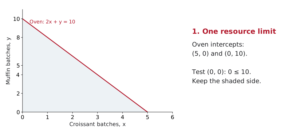
Step 1: draw the oven boundary, then test a side. If you make no muffins, the oven allows \(10/2=5\) croissant batches. With no croissants it allows 10 muffin batches. Join \((5,0)\) to \((0,10)\). The trial point \((0,0)\) uses zero hours, so keep its side of the line, including the boundary.
Step 2: add flour and keep only the overlap. Flour allows 15 croissant batches alone or \(15/3=5\) muffin batches alone. Its line crosses the oven line at \((3,4)\). A plan must satisfy both limits; \((0,10)\) passes the oven test but needs 30 flour units, so it is excluded. Red marks the added boundary.
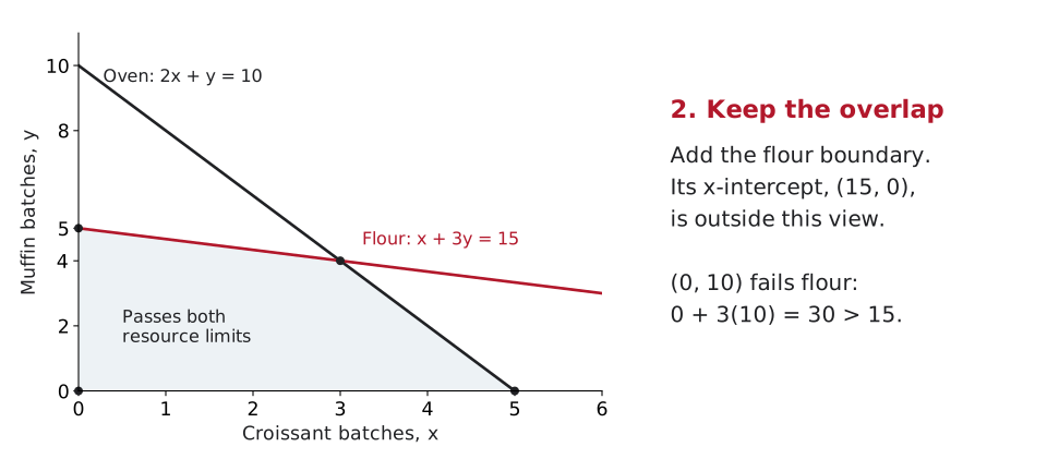
The overlap is the feasible region. Non-negativity keeps it in the first quadrant. Testing a point tells you which side to keep; do not memorize “less than means below” for every possible equation.
Step 3: compare profit without changing the allowed plans. The line \(4x+3y=12\) joins plans earning 12 dollars; \(4x+3y=24\) joins plans earning 24. Their slopes match. Move this line toward higher profit until it last touches the region.
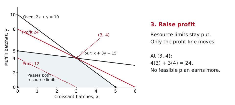
For this bounded, nonempty region, at least one corner attains the best profit. Sometimes an entire edge ties; checking the corners still finds that best value.
Try it: drag the profit slider, then press Maximize and watch where the line stops:
The profit line leaves the region last at the corner where the oven and flour limits cross. That corner is x = 3 croissant batches, y = 4 muffin batches, giving Z = \$24, and the graph proves nothing can beat it.
Build the skill 2: the by-hand method when there is no slider
Away from the widget (on paper, or in an exam) there is no slider. The reliable hand procedure is the corner-point method:
- Plot the constraints, and list the corners of the feasible region.
- Read the \(x\) and \(y\) values at each corner, and compute the objective \(Z\) at each.
- Pick the best, and state the decision in words, with units.
For this bounded feasible region, checking every corner finds the best objective value. For the bakery:
| Corner \((x, y)\) | How it arises | \(Z = 4x + 3y\) |
|---|---|---|
| \((0, 0)\) | both axes (make nothing) | \(0\) |
| \((5, 0)\) | oven line meets \(y = 0\) | \(20\) |
| \((3, 4)\) | oven and flour lines meet | \(\mathbf{24}\) |
| \((0, 5)\) | flour line meets \(x = 0\) | \(15\) |
The corner where the two limits cross comes from solving them together: the oven line gives \(y = 10 - 2x\), so \(x + 3(10 - 2x) = 15\), \(x = 3\), \(y = 4\). And not every place a line meets an axis is a corner: \((0, 10)\), where the oven line meets the \(y\)-axis, would use \(3 \cdot 10 = 30\) units of flour against 15, so it fails the flour limit and sits outside the region. Every corner has to satisfy every constraint.
The biggest \(Z\) is 24 at \((3, 4)\), circle it. Stated in words: bake 3 croissant batches and 4 muffin batches for \$24 profit. That matches the animation exactly, and you can reproduce it with nothing but arithmetic. Drilling this procedure is exactly this week’s graded take-home: the same corner-point tables on two fresh LPs (a campus recycling center and an animal-shelter feed blend) in the starter workbook linked in the take-home section below.
Slack: which resources are you using up?
At a corner, a constraint is either binding (used to the last unit) or has slack: what you had minus what you used, an idle remainder that contributes nothing to profit. Compare the two corners:
- At the optimum \((3, 4)\): oven slack \(= 10 - (2\cdot3 + 4) = 0\) and flour slack \(= 15 - (3 + 3\cdot4) = 0\). Both bind. Every oven hour and every unit of flour is spent. These two binding limits locate this optimum. Other models can have an optimal plan with a resource left over.
- At the corner \((5, 0)\): oven slack \(= 10 - (10 + 0) = 0\) (binding), but flour slack \(= 15 - (5 + 0) = 10\). 10 units of flour sit unused. This plan earns less than the optimum; the unused flour alone does not prove that a plan is inferior.
Monday’s egg limit, \(x + 2y \le 12\), shows the third case. At \((3, 4)\) it reads \(3 + 8 = 11\), so one egg is spare; its tightest point anywhere in the region is that 11 of 12, so the fridge never binds. Monday’s other row, the café’s \(y \ge 2\), is a floor, and \((3, 4)\) bakes 4 muffin batches against the 2 it asks for, so neither row Monday added moves the answer. A limit with slack at the optimum is not holding you back, and paying to raise it (a bigger fridge) buys nothing.
Written in standard form, with a slack variable, the inequality becomes an equation: \(2x + y + s = 10\) with \(s \ge 0\), where \(s\) records the unused oven-hours. Solver does not need the equation: next week you enter the inequality as it stands, and its Answer Report prints the leftover in a column headed Slack. Keep the word in your pocket.
In practice: three ways an LP can surprise you
Most LPs have one tidy corner optimum, like the bakery. But the chapter warns about three irregular cases, and spotting them is a mark of real fluency. Each one can happen to the bakery with a small change to its model:
- Multiple optima. Suppose a croissant batch earned \$6 instead of \$4. The profit line \(6x + 3y\) is three times the oven line \(2x + y\), so it runs exactly parallel to a binding constraint, and pushed outward it leaves the region along a whole edge at once: every plan from \((5, 0)\) to \((3, 4)\) earns \$30, the midpoint \((4, 2)\) included. The corner table shows it as a tie, 30 at both ends of that edge. The model is not broken; you have several equally good answers and can pick among them on something the model left out. Monday’s crisis team ties for the same reason: its \(6x + 9y\) is three times its staff-hours line.
- Infeasible. Suppose the café raised its standing order from 2 muffin batches to 6, \(y \ge 6\). The flour alone caps muffins at \(15 / 3 = 5\) batches, even with no croissants at all, so no plan meets both lines: the feasible region is empty and there is no plan. A requirement has to give, the café’s order or the flour delivery.
- Unbounded. Write the model with the café’s floor, \(y \ge 2\), as its only line: no oven and no flour. Nothing stops one more croissant batch, so profit can climb forever, and the model reports it as unbounded. That is never a real answer. It is a missing-constraint modeling bug, and the kind that announces itself. Drop only the flour line from the original four and the model gives no warning at all: it recommends \((0, 10)\) for \$30, a plan that needs 30 units of flour against 15.
A quick look at minimization (the other half of the chapter)
So far you have maximized profit against \(\le\) limits. Many real problems run the other way: minimize cost subject to requirements you must meet. The morning run has nothing to push inward, because both of its limits are ceilings. The bakery’s catering order brings the floors.
The catering order. An office park has a standing weekly order with the bakery: at least 16 breakfast trays and at least 12 lunch boxes, for a fixed fee. A croissant batch fills 3 trays and 1 box and costs \$5 to bake; a muffin batch fills 1 tray and 3 boxes and costs \$3. The order is baked in the evening, after the morning run, so the morning’s oven hours and flour play no part. What is the cheapest way to fill it?
The fee is fixed, so every dollar saved on baking is a dollar of profit. Same two variables, \(x\) croissant batches and \(y\) muffin batches for the order, and the same three ingredients: the model is \(\min\ 5x + 3y\) subject to \(3x + y \ge 16\) (trays), \(x + 3y \ge 12\) (boxes), \(x, y \ge 0\). Two things flip. (1) The order sets minimums, so the requirements are \(\ge\), and a \(\ge\) keeps the far side of its line: the region sits above the lines and runs off the plot. A profit line pushed outward over that region would never leave it, which is the unbounded case above. So (2) what you push is a cost line, and you push it inward, toward the origin: the last feasible corner it touches is the cheapest, not the richest. The cost line opens at \$60, through the corner \((12, 0)\). Drag the cost slider down, or press Minimize, and watch the line slide toward the origin until it last touches the region (mirror image of the max case):
Now cost every corner of the order, the crossing included:
| Corner \((x, y)\) | How it arises | Cost \(5x + 3y\) |
|---|---|---|
| \((0, 16)\) | tray line meets \(x = 0\) | \(\$48\) |
| \((4.5, 2.5)\) | tray and box lines meet | \(\mathbf{\$30}\) |
| \((12, 0)\) | box line meets \(y = 0\) | \(\$60\) |
The crossing comes from solving the two floors together, as the morning run’s did: the tray line gives \(y = 16 - 3x\), so \(x + 3(16 - 3x) = 12\), \(x = 4.5\), \(y = 2.5\). The two other axis points, \((0, 4)\) and \((5\tfrac{1}{3}, 0)\), are not corners: each falls short of the other floor. Here the crossing wins: bake 4.5 croissant batches and 2.5 muffin batches for \$30. On other problems the minimum sits at an axis corner instead, making none of one product at all, which is exactly why you check every corner rather than assume. This week’s take-home’s shelter blend is one of the other problems: its crossing is not the cheapest corner. Same three-ingredient recipe, mirror-image geometry.
In standard form a \(\ge\) requirement subtracts a surplus variable, the amount above the minimum, to turn the inequality into an equation: \(3x + y - s_{\text{trays}} = 16\) with \(s_{\text{trays}} \ge 0\), where the surplus records trays beyond the 16 ordered. At \((4.5, 2.5)\) both requirements are met exactly, so both surpluses are 0. At \((12, 0)\) the trays come to \(3(12) + 0 = 36\) against 16, a surplus of 20 trays you paid to bake and nobody ordered. Slack is what you had and did not use; surplus is what you delivered and were not asked for. Solver reports both.
A preview: what if you cannot bake half a batch?
That answer asked for 4.5 croissant batches. If the dough can be mixed in half batches, the plan stands as it is. But suppose the mixer takes whole batches only. Every dot below is a whole-batch plan that still fills both floors, and each button draws the cost line through the plan it marks, so any dot on the cheaper side of that line would beat it:
The tempting repair is rounding. It is not reliable. Rounding down to \((4, 2)\) bakes only \(3(4) + 2 = 14\) trays and \(4 + 3(2) = 10\) boxes, short of both floors, so it does not fill the order at all. Rounding up to \((5, 3)\) fills it but costs \$34. The cheapest whole-batch plan is neither: it is \((4, 4)\) at \$32, 16 trays and 16 boxes, which sits on the tray line exactly. Week 10 comes back to this properly, when the whole-number requirement is part of the model rather than an afterthought.
Back to the puzzle
The bakery’s answer is 3 croissant batches and 4 muffin batches, \$24 profit, found two ways that agree: the sliding profit line in the widget, and the corner-point table you can do by hand. You can be sure no plan you never tried does better, because the best plan is always a corner and the table checked all four. Both limits bind, so there is no slack to spare; the plan squeezes every oven hour and every unit of flour. The same picture, turned around, fills the evening’s catering order: floors instead of ceilings, a cost line pushed inward, and 4.5 croissant batches with 2.5 muffin batches for \$30, or \((4, 4)\) for \$32 if the batches must be whole.
Why this matters beyond two variables. Real problems have dozens of variables, and a graph needs one axis per variable, so they are far too many to graph. Next week we hand the same three ingredients to Excel’s Solver, which walks the corners for us and reports the slack on every constraint. The graph is your intuition for what Solver is doing under the hood.
After-class check
Questions spanning model formulation, reading the feasible region and corner points, slack, minimization, and the irregular cases (no feasible solution, unbounded, multiple optima). Retry freely; nothing is submitted.
Weekly take-home (graded: submit on Canvas)
This week’s take-home is two linear programs from two briefs (one maximization for a campus recycling center, one minimization for an animal shelter’s feed blend) and neither model is written down for you. In the Your model block you define the variables with their units and write the objective and every constraint from the narrative, converting one capacity that arrives on the wrong time basis. Then you graph each region. On the maximization you enumerate its corners yourself, with no corner named for you; on the minimization you cost the three candidate corners the workbook lists, and the point where the two lines cross is not the answer. You also identify the constraint that turns out not to matter at all, and the surplus on a minimum the cheapest mix over-delivers. There is no Solver this week. That is Week 8. Two short responses plus the required AI-use disclosure go on the Free responses sheet. Upload the completed .xlsx on Canvas. That one file is your entire submission.