Week 10: Transportation, Transshipment & Assignment
This week’s big question: you have factories that can supply goods and stores that demand them, and a different cost to ship along every route. Which shipping plan meets all the demand at the lowest total cost? These are still linear programs, but they have so much structure that Solver cracks them fast.
These three models run the quiet machinery of the economy: supply networks routing product from plants to stores, crew or shift assignment putting the right person on the right job, machine-to-task scheduling on a factory floor, even matching officials to games. All of them reduce to the same idea. Choose how much flows on each route to hit every requirement at the least total cost.
Before the week
Read: Taylor, Introduction to Management Science (13e), Chapter 6, pp. 261–279, then Chapter 5, pp. 208–220. Chapter 6 carries Monday’s model and Wednesday’s two special cases; Chapter 5 carries Monday’s whole-number section. Both chapters demonstrate two software packages this course does not use, so the real load is about twenty pages. The chapter PDFs are in Canvas Files.
| Pages | Section | This week |
|---|---|---|
| 261–264 | The Transportation Model | Read. Balanced first, then unbalanced (p. 263), which the take-home needs |
| 264–269 | Computer Solution of a Transportation Problem | Read the Excel pages, 264–266. Skip Excel QM (p. 266) and QM for Windows (p. 268) |
| 269–274 | The Transshipment Model | Read. Wednesday: the flow-balance constraint at a hub |
| 274–279 | The Assignment Model | Read pp. 274–276. Skip Excel QM (p. 276) and QM for Windows after it |
| 208–211 | Chapter 5: Integer Programming Models | Read. Total, 0–1, and mixed models, one example each |
| 211–213 | Integer Programming Graphical Solution | Read. Why rounding the LP answer fails, on a picture |
| 213–220 | Computer Solution of Integer Programming Problems | Skim the Excel pages (213–214, 218–220) for the int and bin constraints; skip QM |
Stop where Chapter 6’s Summary begins on p. 279, and at p. 220 in Chapter 5.
Then the warm-up self-check, on supply, demand, and reading a cost matrix:
Session 1: Mon, Oct 26 · Transportation basics and the rounding check
We start with a 30-minute instructor lesson on the shipping grid and why rounding a vehicle purchase can fail. The TA then facilitates 35 minutes of group practice. Photograph your attempt during the next two minutes; the instructor leads the final eight-minute walkthrough.
🧩 Puzzle
One company, two plants, two stores. Plant A can ship 120 units and Plant B can ship 80 (total supply 200). Store 1 needs 100 and Store 2 needs 100 (total demand 200, so the problem is balanced). Shipping costs per unit are: A→Store 1 = \$8, A→Store 2 = \$6, B→Store 1 = \$5, B→Store 2 = \$9. What shipping plan meets every store’s demand at the minimum total cost?
Build the skill 1: set up the transportation grid
First put the brief into a grid. Each inside cell is a cost per unit, not a quantity to ship.
| Cost per unit | Store 1 | Store 2 | Supply |
|---|---|---|---|
| Plant A | 8 dollars | 6 dollars | 120 units |
| Plant B | 5 dollars | 9 dollars | 80 units |
| Demand | 100 units | 100 units | 200 units |
Build a feasible plan before pricing it. Try sending 60 units from A to Store 1. A has 60 left for Store 2; Store 1 still needs 40 from B; B then has 40 left for Store 2. Every row and column now balances.
| Shipment quantity | Store 1 | Store 2 | Row check |
|---|---|---|---|
| Plant A | 60 | 60 | \(60+60=120\) |
| Plant B | 40 | 40 | \(40+40=80\) |
| Column check | \(60+40=100\) | \(60+40=100\) | all demand met |
Price each route using its own cell: \(60(8)+60(6)+40(5)+40(9)=1{,}400\) dollars. This plan works; optimization will ask whether another balanced grid costs less.
A transportation model has a set of sources (each with a fixed supply), a set of destinations (each with a fixed demand), and a unit cost to ship along every source→destination route. The decision variables are the shipment quantities \(x_{ij}\), units sent from source \(i\) to destination \(j\). The objective is to minimize total cost \(\sum_{i}\sum_{j} c_{ij}\,x_{ij}\), subject to “ship out all of each supply” and “meet all of each demand.”
When total supply equals total demand the problem is balanced, and every unit shipped out arrives somewhere. The widget opens on a plan that sends 60 units down the Plant A→Store 1 route, at a cost of \$1,400. Drag the slider to choose how much travels on that route and watch every other route adjust automatically, then hit “Least cost”:
The model, written out
On the puzzle’s numbers the grid is four variables and four equalities:
| Ingredient | In symbols | From the brief |
|---|---|---|
| Decision variables | \(x_{A1}, x_{A2}, x_{B1}, x_{B2}\) | units on each of the four routes |
| Objective | minimize \(8x_{A1} + 6x_{A2} + 5x_{B1} + 9x_{B2}\) | cost grid times shipment grid |
| Supply rows | \(x_{A1} + x_{A2} = 120\); \(x_{B1} + x_{B2} = 80\) | everything each plant ships |
| Demand columns | \(x_{A1} + x_{B1} = 100\); \(x_{A2} + x_{B2} = 100\) | everything each store receives |
The full balanced transportation model is short enough to write in three lines, and these are exactly the families of cells you will type into Solver:
\[\begin{aligned} \text{Minimize } &\sum_{i}\sum_{j} c_{ij}\,x_{ij} \\ \text{subject to } &\sum_{j} x_{ij} = s_i && (\text{each source } i), \\ &\sum_{i} x_{ij} = d_j && (\text{each destination } j), \\ &x_{ij} \ge 0. \end{aligned}\]One supply equality per source row (“everything Plant \(i\) ships sums to its supply \(s_i\)”), one demand equality per destination column (“everything arriving at store \(j\) sums to its demand \(d_j\)”), and shipments can’t go negative. That is the whole model, Solver just searches the \(x_{ij}\) for the cheapest combination that satisfies all the equalities at once.
In Solver the objective cell is one SUMPRODUCT of the two grids: it multiplies the cost grid and the shipment grid cell by cell and adds the results. Each equality is one constraint row.
Build the skill 2: one degree of freedom, so trade cheap routes against dear ones
Notice you only got to choose one number. With 2 sources and 2 destinations there are four routes, but the supply and demand constraints lock down the other three the moment you fix the first. A balanced 2×2 problem has exactly one degree of freedom. Call the units on Plant A→Store 1 \(t\) and watch the constraints force the rest. Row A ships 120, so A→Store 2 is \(120 - t\). Column 1 takes 100, so B→Store 1 is \(100 - t\). Row B ships 80, so B→Store 2 is \(80 - (100 - t) = t - 20\), and it cannot go below zero. Add up the four routes’ costs and the total is
\[8t + 6(120 - t) + 5(100 - t) + 9(t - 20) = 6t + 1{,}040 ,\]a straight line rising \$6 for every unit you push onto the free route. So the whole job is: push flow onto the cheap routes and starve the expensive ones, as far as the supplies and demands allow. The floor is \(t = 20\): any lower and B→Store 2 goes negative. Ship 20, 100, 80, 0 for \$1,160, with the cheap \$5 route running flat out and the dear \$9 route empty. Plant B only has 80 units, so it sends all 80 to Store 1; the remaining 20 of Store 1’s demand must come from Plant A, and that forces the rest of the grid.
Build the skill 3: when the answer has to be a whole number
Look again at the plans you just built. Every shipment came out a whole number of units and nobody had to ask for it. On the 2×2 you can see why: the free number \(t\) is legal from 20 (where B→Store 2 hits zero) to 100 (where B→Store 1 hits zero), both ends are whole because they came from whole supplies and demands (\(100 - 80 = 20\), and 100), and the best plan sits at an end. The structure handed you integers for free, and it is the same structure that lets Solver dispatch large grids in a blink. Now take that structure away.
The company plans to add Plant C and Store 3 and is buying vehicles for the expansion. A box truck costs \$60,000, needs 1 driver, and moves 5,000 units a month. A cargo van costs \$40,000 and runs two shifts, so it needs 2 drivers, and moves 4,000. There is \$240,000 to spend and 6 drivers to assign. Counting the budget in \$10,000 units and capacity in thousands of units a month, with \(x\) box trucks and \(y\) cargo vans:
\[\text{Maximize } 5x + 4y \quad\text{s.t.}\quad 6x + 4y \le 24 \ (\text{budget}),\quad x + 2y \le 6 \ (\text{drivers}),\quad x, y \ge 0 .\]First allow fractional vehicles and solve the resulting LP: draw the two lines, shade what survives both, and go to a corner. The budget line runs from \((4, 0)\), four box trucks and nothing else, to \((0, 6)\); the driver line from \((0, 3)\), three vans using every driver, to \((6, 0)\). They cross at \(x = 3\), \(y = 1.5\), and that corner moves \(15 + 6 = 21\) thousand units a month. There is no such thing as half a van. Solving the problem while ignoring the whole-number requirement is called the LP relaxation, and its answer is a ceiling: the true whole-number plan can never beat it.
The obvious repair is to round. Try it below. Every dot is a whole-number plan that fits inside both the budget and the drivers:
Rounding up to \((3, 2)\) breaks both constraints at once: \$260,000 against a \$240,000 budget, and 7 drivers out of 6. Rounding down to \((3, 1)\) is affordable at \$220,000 and moves 19,000 units a month, which is legal but not the best you can do. The real optimum is \((4, 0)\): four box trucks and no vans at all, spending the \$240,000 exactly and moving 20,000 units a month.
The whole-number answer uses a different mix from either rounded plan. On Wednesday we distinguish integer-model types and add the whole-number restrictions in Solver. Today’s handout uses the same check: test both limits and compare feasible whole-number plans.
Back to the puzzle
The minimum-cost plan ships 20 on Plant A→Store 1 (so A→Store 2 = 100, B→Store 1 = 80, B→Store 2 = 0), for a total cost of \$1,160, the lowest the slider can reach. Check it: \(20(8) + 100(6) + 80(5) + 0(9) = 160 + 600 + 400 + 0 = 1{,}160\). The intuition pays off: cheap B→Store 1 runs flat out, expensive B→Store 2 carries nothing, and Plant A quietly covers what’s left. Wednesday asks the same network two new questions: whether a hub between the plants and the stores can beat \$1,160, and which crew should take each store’s delivery run.
In-class group practice (wrap-up)
To close Session 1, find a low-cost shipping plan and compare whole-number vehicle plans by hand in your group.
Write every member’s name on the sheet. You have 35 minutes with the TA for the practice, then two minutes to photograph your group’s own attempt before the solutions are shown. One member uploads the photo to Canvas by the end of class; participation credit is for attempting the work.
The instructor uses the final eight minutes to demonstrate the handout’s method, check the main results with units, and explain a common mistake. This demonstration closes the session.
- Download: Week 10 group practice (Word)
Session 2: Wed, Oct 28 · Transshipment & assignment (special cases)
🧩 Puzzle
Same company, two new questions. The company opens a hub between Plants A and B and Stores 1 and 2. Trucking a unit into the hub costs \$2 from either plant, and sending it on costs \$4 to Store 1 and \$3 to Store 2; Monday’s four direct routes stay open at Monday’s costs. Should Monday’s 200 units go direct, through the hub, or some of each, and what does the best plan cost? Each store’s delivery run also needs a crew: Crew 1 takes 7 hours on the Store 1 run and 9 on the Store 2 run; Crew 2 takes 8 and 5. Each crew takes exactly one run and each run needs exactly one crew. Which crew should take which run?
Extend the grid and make whole-number requirements explicit
Monday’s two-plant grid grows before we add the hub and the delivery crews. The same company carries all of today’s extensions, including the distinction between naturally whole shipment quantities and decisions that need an explicit integer restriction.
Now scale it past what you can eyeball
A 2×2 has one free number. You really can do it in your head. Real problems are not 2×2, and the company is growing: it opens Plant C (100 units) and Store 3 (100 units), so three plants (120, 80, 100; total 300) ship to three stores (100 each; total 300, still balanced), with a unit cost for every route. The puzzle’s four costs sit in the top-left corner, and each plant’s cheapest store is in bold:
| \$ per unit | Store 1 | Store 2 | Store 3 | Supply |
|---|---|---|---|---|
| Plant A | 8 | 6 | 4 | 120 |
| Plant B | 5 | 9 | 7 | 80 |
| Plant C | 3 | 4 | 5 | 100 |
| Demand | 100 | 100 | 100 |
Now there are nine routes and four degrees of freedom. Try the obvious shortcut first: give every plant its cheapest store. Plant A would send all 120 to Store 3, which wants 100; Plants B and C would both pile onto Store 1, 180 units for a store that wants 100; and Store 2 would get nothing. Where the leftovers go is the whole problem, and there are far too many combinations to eyeball. Type this grid into Solver with the three supply equalities and three demand equalities and it returns the plan in well under a second: Plant A ships 20 to Store 2 and 100 to Store 3, Plant B sends all 80 to Store 1, and Plant C ships 20 to Store 1 and 80 to Store 2, at a total cost of \$1,300. Check it:
\[20(6) + 100(4) + 80(5) + 20(3) + 80(4) = 120 + 400 + 400 + 60 + 320 = 1{,}300 .\]Plant B’s plan is the puzzle’s; Plant A has left Store 1 to Plant C. That is the whole reason for Solver: same skill as the 2×2 (read the grid, write the equalities, minimize the cost sum), but now with too many routes to guess.
The larger shipment grid still has a whole-number optimum because of its network structure. The vehicle purchase needs a different rule: its best whole-number mix, four trucks and no vans, differs from both roundings of the fractional plan. Integer programming is what you use when the decision variables have to come out whole, and Taylor splits the models three ways by which variables carry the requirement: a total integer model where every variable is whole (how many box trucks, how many vans), a 0-1 model in which each decision is a binary variable, 1 for yes and 0 for no (whether to open Plant C at all), and a mixed-integer model where some variables are whole and others stay continuous (open Plant C or not, then ship any amount from it).
In Solver the change is one line. Add a constraint on the decision cells whose relation is int, or bin for yes/no. What it costs you is speed. Solver can no longer slide along the edges of the region to a corner; it has to search among the dots, which it does by branch and bound, repeatedly solving relaxed LPs and discarding whole branches that cannot beat the best whole-number answer found so far. At this size that is instant. It is also why integer models scale worse than the transportation model you just built, whose structure hands you whole units without paying that cost at all.
Build the skill 1: transshipment: pass-through nodes in the middle
A transshipment model is a transportation model with intermediate nodes. Think a port, warehouse, or hub between the sources and the destinations. Goods can flow source → hub → destination instead of going direct, and a hub is neither a final source nor a final sink: whatever flows in must flow out. That is a flow-conservation constraint, and it is a real equation, not just a slogan.
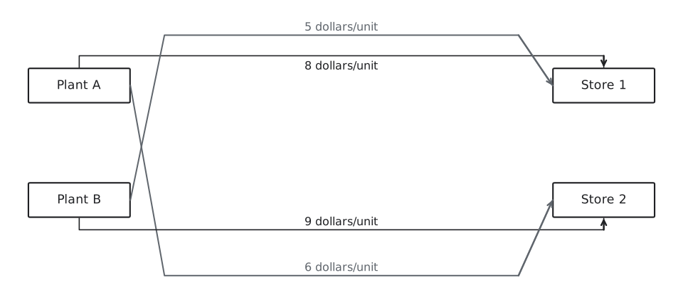
1. Keep the direct routes visible. These are the four original routes, labelled in dollars per unit.
2. Add the hub and its four legs in red. A route through the hub pays once to enter and once to leave. The direct routes remain available.
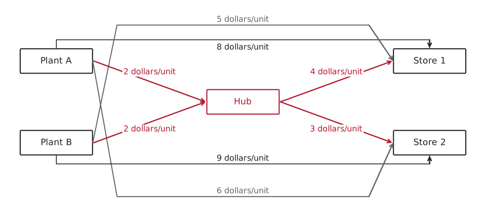
The puzzle’s hub gives every unit two ways to reach a store. Start with the two pure plans. Direct only is Monday’s answer: 20, 100, 80 and 0 units on the four routes, for \$1,160. Everything through the hub pays two legs on every unit, \$2 in and then \$4 or \$3 out:
\[120(2) + 80(2) + 100(4) + 100(3) = 240 + 160 + 400 + 300 = 1{,}100 .\]For this all-hub trial, all 200 units that arrive must leave. Its numeric balance is
\[\underbrace{120 + 80}_{\text{into the hub}} \;=\; \underbrace{x_{H1} + x_{H2}}_{\text{out of the hub}} \;=\; 200 .\]The compact check is \(\text{inflow}=\text{outflow}\) at a pure transfer node.
With both open, each plant has two paths to each store. The hub has no capacity limit here, so nothing stops a unit from taking the cheaper one:
| Plant → store | Direct | Through the hub | Cheaper |
|---|---|---|---|
| A → Store 1 | \$8 | \$2 + \$4 = \$6 | hub |
| A → Store 2 | \$6 | \$2 + \$3 = \$5 | hub |
| B → Store 1 | \$5 | \$2 + \$4 = \$6 | direct |
| B → Store 2 | \$9 | \$2 + \$3 = \$5 | hub |
That is Monday’s 2×2 again, with the cheaper path’s cost on each pair (6, 5, 5 and 5), and Monday’s free number finishes it. With \(t\) units going from Plant A to Store 1, the total is \(6t + 5(120 - t) + 5(100 - t) + 5(t - 20) = t + 1{,}000\), still lowest at \(t = 20\). So Plant B’s 80 units go straight to Store 1, and all 120 of Plant A’s go through the hub, 20 on to Store 1 and 100 on to Store 2:
\[80(5) + 120(2) + 20(4) + 100(3) = 400 + 240 + 80 + 300 = 1{,}020 .\]3. Put the chosen quantities on the network. Red marks the selected flows; each label multiplies units by dollars per unit.
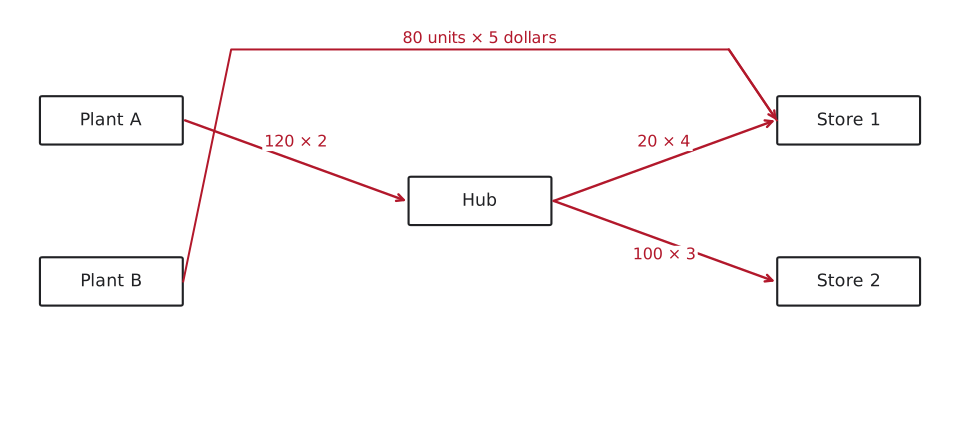
The hub balances on these flows too, with 120 units in from Plant A, none from Plant B, and 20 and 100 out:
\[\underbrace{120 + 0}_{\text{into the hub}} \;=\; \underbrace{20 + 100}_{\text{out of the hub}} \;=\; 120 .\]For any plan, name the four hub flows before writing its balance: \(x_{AH}\) and \(x_{BH}\) enter from the plants, while \(x_{H1}\) and \(x_{H2}\) leave for the stores. The model adds
\[x_{AH}+x_{BH}-x_{H1}-x_{H2}=0.\]The chosen plan makes this \(120+0-20-100=0\). The equation keeps the same meaning while Solver changes the four shipment quantities.
In Solver that balance is one cell: everything inbound minus everything outbound, constrained to equal 0. Leave it out and the hub can hand out goods it never received. Write the plants’ rows as \(\le\), which on Monday’s grid changed nothing, and Solver sends all 200 units out of the hub without shipping a single one in: a \$700 plan for goods no plant made.
The routing is flexible: goods can go source → hub → destination, hub → hub (one hub forwarding to another), or source → destination directly, skipping the hub, as Plant B’s units do. A hub is an option, not a forced detour. Why have hubs at all? Consolidation: pooling many small shipments at a hub can make the per-leg cost low enough that hub routing beats shipping direct, which is exactly why freight networks are built around them. Plant B’s row shows the converse: \$2 in plus \$4 out comes to \$6, a dollar more than its \$5 direct run to Store 1, so for that pair the hub does not pay for itself. A hub is worth running only while the saving on the legs beats the extra handling. Solver handles all of this with the same minimize-cost setup, just more nodes and one flow-balance equation at each hub.
Build the skill 2: assignment: a transportation problem where everything equals 1
The goods now have routes; the remaining choice is who makes each delivery. This is a separate matching decision, measured in crew-hours, so do not add these hours to the shipping dollar totals.
| Hours for one run | Store 1 run | Store 2 run |
|---|---|---|
| Crew 1 | 7 | 9 |
| Crew 2 | 8 | 5 |
Circle one cell in every row and every column. The diagonal pairing totals \(7+5=12\) hours; the other pairing totals \(9+8=17\). Those row and column rules will become the model’s constraints.
An assignment model is the cleanest special case: every source has supply 1 and every destination has demand 1. You’re not splitting shipments. You’re matching each crew to exactly one run (the same model puts each machine on one task, or each official on one game). Formally each xᵢⱼ ∈ {0, 1} (\(1\) if crew \(i\) takes the run to store \(j\), else \(0\)), and the constraints are simply
One crew per row, one run per column. Notice Solver returns clean 0s and 1s here without being told to, the same free integrality you met on Monday: the network structure does it, not an int constraint.
Two crews give two matchings, and you can cost both by hand. Crew 1 on the Store 1 run with Crew 2 on the Store 2 run is \(7 + 5 = 12\) hours; the cross assignment, Crew 1 on Store 2’s run and Crew 2 on Store 1’s, is \(9 + 8 = 17\). And there is one free number, exactly like Monday’s \(t\): set \(x_{11} = 1\) and the other three cells are forced (\(x_{12} = 0\), \(x_{21} = 0\), \(x_{22} = 1\)). Slide the free route and watch the readout report 17 hours at \(x = 0\) and 12 at \(x = 1\); hit “Least cost” and the optimal matching locks in at \(x = 1\):
Why you cannot eyeball the big ones
Two crews give just 2 possible matchings, easy. Now the company’s other two crews join, and two more runs need a crew each: the new Store 3 from today’s larger grid, and the hub run that trucks goods from the plants into the hub. Hours as before, with the puzzle’s 7, 9, 8, 5 in the top-left corner. The optimal matching is in bold:
| Hours | Store 1 run | Store 2 run | Store 3 run | Hub run |
|---|---|---|---|---|
| Crew 1 | 7 | 9 | 5 | 3 |
| Crew 2 | 8 | 5 | 4 | 8 |
| Crew 3 | 12 | 12 | 7 | 5 |
| Crew 4 | 12 | 11 | 5 | 8 |
The tempting move is to grab the single smallest cell (Crew 1 on the hub run, 3 hours), then the cheapest of what is left. Do that greedily: Crew 2 on the Store 3 run (4), then Crew 4 on the Store 2 run (11), and Crew 3 is left with the Store 1 run (12), for a total of 30 hours. But the true optimum never touches that 3-hour cell at all: Crew 1 on Store 1 (7), Crew 2 on Store 2 (5), Crew 3 on the hub run (5), Crew 4 on Store 3 (5) = 22 hours, eight hours less, and the puzzle’s own matching is still inside it. Eyeballing fails because the cheapest individual choice can poison the rest of the grid, and the shortcut gets worse as the grid grows, because every early grab removes a row and a column from everyone else’s options. With four crews there are \(4! = 24\) matchings to weigh; bump it to ten crews and ten runs and there are \(10! = 3{,}628{,}800\), about 3.6 million. Nobody checks 3.6 million by hand. You need the model and Solver.
Three models, one Solver pattern
| Transportation | Transshipment | Assignment | |
|---|---|---|---|
| Variables | units on each route | units on each arc, hubs included | 0 or 1 on each pairing |
| Constraints | row \(=\) supply, column \(=\) demand | the same, plus in \(=\) out at every hub | every row and column \(= 1\) |
| Objective | SUMPRODUCT of cost and flow | the same, over every arc | the same, over every pairing |
| Whole units | free, from the structure | free | free: clean 0s and 1s |
Learn one and the other two are a change of right-hand sides and one extra equation. That table is the take-home.
In practice: real shipping problems rarely arrive this tidy
- Unbalanced totals flip the constraint type. When supply exactly equals demand, the supply and demand constraints are equalities (\(=\)). When they don’t match, Taylor’s rule is to switch the larger side’s constraints to \(\le\): if supply > demand, the supply constraints become \(\le\) (some supply stays put); if demand > supply, the demand constraints become \(\le\) (some demand goes unmet). An equivalent reformulation is to rebalance with a dummy node. Supply > demand → a dummy destination absorbs the excess at \$0 cost; demand > supply → a dummy source “covers” the shortfall on paper (the demand it fills is really unmet). Both give the same plan; in Solver it is just the difference between an \(=\) and a \(\le\) on the relevant constraint. Two habits go with this. Compare the totals in the same unit first: a demand quoted in cases and a supply counted in pallets cannot be compared until one is converted. And read the dummy column afterwards, because it tells you which source holds stock back, and how much. If Plant B could ship 100 instead of 80, supply would be 220 against demand of 200. A dummy store takes the extra 20, and the cheapest plan (Plant B’s 100 to Store 1, 100 of Plant A’s to Store 2, \$1,100) puts all 20 in the dummy column on Plant A’s row: Plant A is the one holding stock back.
- Costs aren’t always per unit. A carrier may charge per truck or per trip, or give volume discounts, then the cost is no longer a clean \(c_{ij}\) per unit and the plain transportation model needs adjusting.
- Transportation hands you whole units. Most models do not. Because the supplies and demands are whole numbers here, the optimum lands on whole units by itself, and that same network structure is why Solver dispatches even large transportation problems so quickly. When a model has no such structure, never round a fractional answer and call it done: rounding can land you outside the feasible region, and even when it stays inside it can miss the best whole-number plan, exactly as it did with the trucks and vans. Say
intorbinin the model and let Solver search.
In practice: small grids are deceiving; the model is what scales
- The greedy “grab the cheapest cell” rule is wrong, as the 4×4 above showed. Handing each crew its own fastest run fails the same way: Crews 1 and 3 both want the hub run, and Crews 2 and 4 both want Store 3’s. Assignment optimizes the whole matching at once, which is why you let Solver do it instead of picking cells by hand.
- Make it square first. Assignment assumes equal numbers of crews and runs. More runs than crews? Add a dummy crew (with large or zero “do-nothing” costs) so the model stays balanced. The unfilled run just gets the dummy. This is the assignment version of the dummy-source / dummy-destination rule above.
- The costs encode your real goal. Put hours in the grid and you minimize time; put dollars and you minimize money; put a “happiness” penalty and you can model preferences. The math doesn’t care, so make sure the numbers you feed it mean what you intend.
Back to the puzzle
Use the hub and the direct routes together. Plant B’s 80 units go straight to Store 1, and all 120 of Plant A’s go through the hub, 20 on to Store 1 and 100 on to Store 2, for \$1,020, against \$1,160 direct only and \$1,100 through the hub only. The hub takes in 120 units and sends out 120, and in Solver that balance is the one cell the hub adds. For the runs, Crew 1 takes the Store 1 run and Crew 2 the Store 2 run: \(7 + 5 = \textbf{12}\) hours, against 17 for the cross assignment, exactly where the slider’s “Least cost” button lands. Same minimize-cost idea as Session 1: a hub adds one equation, and a matching is the special case where every supply and demand equals 1, small enough here that both matchings can be costed by hand. At four crews the hand method already fails (the greedy grab costs 30 hours against 22). At ten it is not an option.
After-class check
Questions spanning the transportation model, balancing with a dummy source/sink, whole-number decisions, transshipment hubs, and assignment as a 1-to-1 special case. Retry freely; nothing is submitted.
Weekly take-home (graded: submit on Canvas)
Everything for the take-home lives in one Excel workbook, and it builds all three of this week’s models with the same Solver pattern. The first brief is a book distributor whose depot stock is counted in pallets while its zones order in cases, and once you convert them, supply and demand do not balance, so you have to repair the model before it will solve at all. The second is a library sending three auditors to three branches: try the obvious shortcut of giving each auditor their own fastest branch and watch it collide, then build the 0/1 grid properly. The third is a food-bank cross-dock, where you write the flow-balance condition yourself and then solve the network three ways (direct only, through the dock only, and with both available) to see which wins and which pantry stays direct. Solver fills the shipment grids; the conversions, the formulas and the repair are yours. Three short responses plus the required AI-use disclosure go on the Free responses sheet. Upload the completed .xlsx on Canvas. That one file is your entire submission.