Week 11: Multi-Criteria Decision Making & Goal Programming
This week’s big question: real decisions almost never have a single number to maximize. You care about cost and quality and time and space, goals that pull against each other. How do you turn several competing criteria into one defensible choice?
Before the week
- Read: Taylor, Introduction to Management Science (13e): Chapter 9, “Multicriteria Decision Making,” pp. 443–469 (focus: goal programming with deviation variables, and weighted / AHP-style scoring). What we call weighted scoring the book files under “Scoring Models” on p. 467.
- Warm-up self-check, weighted averages and comparing scores on different scales:
Session 1: Mon, Nov 2 · Scoring across many criteria (TBD)
🧩 Puzzle
The legal-aid nonprofit’s new office. A small legal-aid nonprofit is choosing among three office sites and cares about three things: the monthly cost of the rent (cheaper is better), access by public transit, which its clients depend on, rated 1–10 (higher is better), and usable space (more is better).
Site Cost (monthly rent) Transit access (1–10) Usable space (m²) A \$1,300 8 40 B \$1,000 6 30 C \$1,600 9 55 Site B is the cheapest, but also the most cramped and the hardest to reach by bus. Site C is the roomiest and the best connected, but it costs the most. Site A sits in the middle on all three. No site wins on everything, so which one do you pick?
Build the skill 1: put every criterion on the same 0–1 scale
The trouble is that cost is in dollars, access is a 1–10 rating, and space is in square meters. You can’t add them directly. So first normalize each criterion onto a common 0–1 scale, where 1 = best and 0 = worst for that criterion. For a “higher is better” criterion like space, the biggest value maps to 1; for a “lower is better” criterion like cost, the smallest value maps to 1. The standard recipe is min–max: take \((\text{value} - \min) / (\max - \min)\), and for a lower-is-better criterion subtract the result from 1. On the puzzle’s table:
- Cost (lower better): A \(\to 1 - (1{,}300 - 1{,}000)/(1{,}600 - 1{,}000) = 0.5\), B \(\to\) 1.0, C \(\to\) 0.0
- Access (higher better): A \(\to (8 - 6)/(9 - 6) = 2/3 \approx 0.67\), B \(\to\) 0.0, C \(\to\) 1.0
- Space (higher better): A \(\to (40 - 30)/(55 - 30) = 0.4\), B \(\to\) 0.0, C \(\to\) 1.0
Keep the original measurements beside the converted scores. A zero means worst among these three sites on this criterion, not “no access” or “no space.”
| Site | Rent (dollars/month) → score | Access rating → score | Space (m²) → score |
|---|---|---|---|
| A | 1,300 → 0.50 | 8 → \(2/3\) | 40 → 0.40 |
| B | 1,000 → 1.00 | 6 → 0.00 | 30 → 0.00 |
| C | 1,600 → 0.00 | 9 → 1.00 | 55 → 1.00 |
For example, A is halfway between the cheapest and most expensive rents, so its cost score is 0.50. Its access is two of the three rating points from 6 to 9, so its access score is \(2/3\). Keep that fraction until the final total to avoid rounding the ranking early.
Now every number lives on the same ruler and the criteria are finally comparable.
Build the skill 2: weight, sum, and watch the winner flip
Not every criterion matters equally, so give each one a weight, with the weights summing to 1, multiply each normalized score by its weight, and add them up to a single weighted score for each site. With weights Cost 0.5, Access 0.3, Space 0.2 the totals come out close:
- Site A \(= 0.5(0.5) + 0.3(2/3) + 0.2(0.4) = 0.25 + 0.20 + 0.08 = \mathbf{0.53}\)
- Site B \(= 0.5(1.0) + 0.3(0.0) + 0.2(0.0) = \mathbf{0.50}\)
- Site C \(= 0.5(0.0) + 0.3(1.0) + 0.2(1.0) = \mathbf{0.50}\)
So Site A wins, but only barely. Drag the weight sliders and watch the ranking. Raise Space from 0.20 to 0.30, or Access from 0.30 to 0.40, and the winner flips to Site C; raise Cost from 0.50 to 0.60 and Site B takes over. The widget divides the three sliders by their total, so the weights it uses always sum to 1, and it reads each score as a percentage, so Site A’s 0.53 shows as 53%.
That fragility is the lesson: when scores are this close, the “winner” is really a statement about your weights, not a fact about the sites.
A second, simpler way to score (Taylor’s scoring model). Min–max normalization is one option, but the textbook’s everyday scoring model skips it: a team just grades each option 0–100 on each criterion (their own honest judgment) and uses weights that sum to 1, so \(\text{score}_i = \sum_j w_j\, g_{ij}\) with \(w_j \in [0,1]\) and \(g_{ij}\) a 0–100 grade. Say the nonprofit’s staff grade the three sites on cost, access and space: Site A 70, 80, 60; Site B 90, 60, 45; Site C 50, 90, 90. With the same weights, Site A scores \(0.5(70) + 0.3(80) + 0.2(60) = 35 + 24 + 12 = \mathbf{71}\), Site B \(45 + 18 + 9 = \mathbf{72}\) and Site C \(25 + 27 + 18 = \mathbf{70}\), so Site B wins, where min–max crowned Site A. The grades rank the sites in the same order as the table on every criterion; what differs is the spacing. Min–max stretches each column to fill 0 to 1, so Site B’s transit rating of 6, the worst of the three, becomes a zero, while the staff grade the same access 60 out of 100. Grading is faster than normalizing and is what most real scorecards use, but the grades are pure judgment, which is exactly why you must disclose your method: the two scales just crowned different winners from the same three sites.
Where the weights come from: AHP
Both methods above just assert the weights (Cost 0.5, Access 0.3, Space 0.2) as if they fell from the sky. The Analytical Hierarchy Process (AHP) derives them from stated pairwise comparisons. They remain judgments; AHP makes their relationships checkable. You only ever answer one question at a time: “comparing just these two, how much more important is this one?”, scored on Taylor’s 1–9 preference scale, where \(1\) is equally preferred, \(3\) moderately, \(5\) strongly, \(9\) extremely, the even numbers sit in between, and the reciprocal (\(1/5\)) records the case where the other one wins.
Say the nonprofit’s board rates cost a notch above equal against access (\(2\)), cost a notch above equal against space (\(2\)), and access a notch above equal against space (\(2\)). Each judgment fills one cell, and its reciprocal fills the mirror cell:
| Board’s comparisons | Cost | Access | Space |
|---|---|---|---|
| Cost | 1 | 2 | 2 |
| Access | 1/2 | 1 | 2 |
| Space | 1/2 | 1/2 | 1 |
| Column sum | 2 | 3.5 | 5 |
Divide each entry by its column sum, then average each row. The row averages are the criteria’s preference vector, their weights, and they sum to 1:
| Divided by column sum | Cost | Access | Space | Row average (weight) |
|---|---|---|---|---|
| Cost | 0.5000 | 0.5714 | 0.4000 | 0.4905 |
| Access | 0.2500 | 0.2857 | 0.4000 | 0.3119 |
| Space | 0.2500 | 0.1429 | 0.2000 | 0.1976 |
For the cost row, the three normalized entries average to \((0.5000+0.5714+0.4000)/3\approx0.4905\). Repeat for access and space. This column-normalize-and-average procedure is the approximation used here; the matrix supplies weights, while the site’s normalized performance scores still come from the earlier table.
The board has said cost is twice as important as access and access twice as important as space. Perfect consistency would therefore make cost four times as important as space, but its direct judgment was two. The next check measures how serious that mismatch is; it does not test whether the board chose the “right” values.
Before trusting those weights, AHP checks that the judgments hang together. Multiply the comparison matrix by the weights and divide each result by its own row’s weight. For cost, \(1(0.4905) + 2(0.3119) + 2(0.1976) = 1.5095\), and \(1.5095 / 0.4905 = 3.08\); access and space give 3.05 and 3.03. A perfectly consistent board would get exactly 3, the number of items compared, on every row, and these average 3.054. The excess becomes the consistency index, \(\text{CI} = (3.054 - 3)/(3 - 1) = 0.027\), and the consistency ratio compares it with the random index RI, the average CI of randomly filled matrices, which Taylor tabulates as 0.58 for three items:
\[\text{CR} = \text{CI} / \text{RI} = 0.027 / 0.58 \approx 0.05.\]Taylor’s rule of thumb accepts a ratio under 0.10, so the board’s weights stand. Put them in place of 0.5, 0.3 and 0.2 and Build the skill 1’s normalized scores give Site A 0.53, Site C 0.51 and Site B 0.49: the same winner, now earned from comparisons the board made itself. Full AHP goes one step further and scores the sites the same way, one comparison matrix per criterion, whose row averages replace the min–max scores; Taylor works that version through in ch. 9, repeating these steps.
In practice: a single score hides the judgment calls
- Weights are subjective. Cost 0.5 versus Cost 0.4 is a value judgment, not a measurement, and here it decides the office: at 0.4, Site C wins. Always do a sensitivity check: slide the weights and see whether your winner survives. If it flips easily, say so.
- The scale changes the ranking. Min–max crowned Site A and the staff’s 0–100 grades crowned Site B, from the same three sites. Divide-by-max and z-scores are further options, and each can crown a different alternative. Pick one method and disclose it so reviewers can argue about the method, not just the result.
- Are your comparisons even self-consistent? Suppose the board had said cost is strongly more important than access (\(5\)) and access strongly more important than space (\(5\)), yet cost only moderately more important than space (\(3\)). Two strong steps in a row should compound into something far stronger than moderate, so the judgments contradict each other, and the same steps catch it: CI about 0.27 and a consistency ratio of about 0.47, far over 0.10. The weights that fall out, about 0.60, 0.28 and 0.12, would hand the office to Site B on judgments the board itself contradicted, so redo the comparisons. Ad-hoc weights have no such alarm, which is part of why AHP is more defensible.
- Beware false precision. “Site A scored 0.530” looks authoritative, but its lead is 0.03, and one point on one rating erases it: rate Site A’s transit access 7 instead of 8 and its score drops to 0.43, last of the three. Report the close calls instead of hiding them behind a decimal.
Back to the puzzle
At the stated weights the nonprofit should lean toward Site A: it scores 0.53 against 0.50 for both B and C, and the board’s own AHP comparisons agree (0.53 against 0.51 and 0.49). But the honest recommendation is “A, narrowly”: a tenth more weight on space or transit access makes C the better choice, and the staff’s 0–100 grades already put B a point ahead. The weighted-scoring model didn’t make the decision for them; it made the trade-off visible so the board can argue about weights and scales instead of arguing past each other. And if the board distrusts round-number weights, AHP builds them from comparisons it actually believes, and checks that those comparisons agree with each other.
In-class group practice (wrap-up)
To close Session 1, score a set of alternatives by hand in your group.
Write every member’s name on the sheet. You have 15 minutes for the practice, then two minutes to photograph your group’s own attempt before the solutions are shown. One member uploads the photo to Canvas by the end of class; participation credit is for attempting the work.
The instructor uses the final eight minutes to demonstrate the handout’s method, check the main results with units, and explain a common mistake. This demonstration closes the session.
- Download: Week 11 group practice (Word)
Session 2: Wed, Nov 4 · Goal programming (TBD)
🧩 Puzzle
Same nonprofit, new question: the weekly clinic schedule. The legal-aid nonprofit took Site A and now plans its week: \(x\) know-your-rights workshops and \(y\) one-on-one consultations. A workshop runs two hours in the building’s shared community room (the office itself is too small for a group), takes two staff members, so 4 staff hours, and reaches 12 clients. A consultation takes 1 staff hour in the office and serves one client. The director has four targets: use all 40 staff hours a week that the grant pays for, serve at least 80 clients a week, book the community room for no more than the 8 hours a week it is free (a workshop past that goes to a rented room across town), and avoid overtime. They pull against each other: workshops reach more people per staff hour, but the room caps them, and every consultation costs an hour of staff time. What do you do when you can’t hit every target, and some targets matter more than others?
Build the skill 1: turn “soft” targets into deviation variables
In ordinary linear programming you maximize one objective subject to hard constraints. But here the targets are goals, not iron rules. Serving 76 clients instead of 80 isn’t infeasible; it is just short. Goal programming captures that by attaching two deviation variables to each goal: \(d^{+},d^{-}\) for how much you overshoot and undershoot the target, respectively. First check one proposed schedule: 4 workshops and 20 consultations. It uses \(4(4)+20=36\) staff hours, four below the funded 40. To balance “actual plus shortage equals target,” add the missing four:
\[36+4-0=40.\]If the schedule used 48 hours instead, subtract its eight-hour overage: \(48+0-8=40\). This is why a goal constraint always has the form actual + undershoot − overshoot = target.
Build one row at a time. Each deviation has the same unit as its own goal.
| Goal | Actual for any plan | Goal equation | At \((4,20)\) |
|---|---|---|---|
| Staff hours | \(4x+y\) | \(4x+y+d^-_{\text{hours}}-d^+_{\text{hours}}=40\) | \(36+4-0=40\) |
| Clients | \(12x+y\) | \(12x+y+d^-_{\text{clients}}-d^+_{\text{clients}}=80\) | \(68+12-0=80\) |
| Room hours | \(2x\) | \(2x+d^-_{\text{room}}-d^+_{\text{room}}=8\) | \(8+0-0=8\) |
The overtime goal needs no equation of its own: overtime is the staff-hours goal’s overshoot, \(d^{+}_{\text{hours}}\), just as the hours spent in a rented room are the room goal’s overshoot, \(d^{+}_{\text{room}}\). Use nonnegative deviations. When reporting a plan, at least one of its overage and shortage is zero: a realized quantity cannot be both above and below one target. The equation alone permits adding the same amount to both deviations; minimizing unwanted deviations removes that unnecessary excess.
The widget below starts at a first try: four workshops, which fill the room’s 8 hours, and 20 consultations. Staff hours are \(4(4) + 20 = 36\), so \(d^{-}_{\text{hours}} = 4\) and \(d^{+}_{\text{hours}} = 0\); clients are \(12(4) + 20 = 68\), so \(d^{-}_{\text{clients}} = 12\); the room is booked for exactly \(2(4) = 8\) hours, so both room deviations are 0. The readout lists the same misses, goal by goal:
The widget reports each plan as goals met or missed, never “infeasible”, because a missed goal is just a nonzero deviation. Drag the dot. Straight up adds consultations: each one closes the client gap by one and adds a staff hour, so from 24 consultations the staff-hours goal is met, and past 24 the no-overtime goal starts to miss. Sideways moves change the workshops: each one adds 12 clients for only 4 staff hours, but any plan to the right of \(x = 4\) misses the room goal. No plan meets all four goals at once. That is the conflict, and ranking the goals is how you settle it.
Build the skill 2: rank the goals and minimize only the deviations you do not want
Instead of maximizing one number, goal programming minimizes the unwanted deviations. The trick is naming, for each goal, which direction is “bad”:
| Goal type | Example | Undesired deviation | You minimize |
|---|---|---|---|
| at-least (reach a floor) | clients \(\ge\) 80 a week | undershoot | \(d^{-}\) |
| at-most (stay under a cap) | community room \(\le\) 8 hours a week | overshoot | \(d^{+}\) |
When goals conflict, preemptive (priority) goal programming ranks them and writes a lexicographic objective. Satisfy Priority 1 as well as possible, then, without sacrificing it, work on Priority 2, and so on. The director ranks the four goals in the order the puzzle listed them:
- P1: use all 40 funded staff hours: minimize \(d^{-}_{\text{hours}}\)
- P2: serve at least 80 clients: minimize \(d^{-}_{\text{clients}}\)
- P3: keep workshops within the community room’s 8 free hours: minimize \(d^{+}_{\text{room}}\)
- P4: avoid overtime past the 40 staff hours: minimize \(d^{+}_{\text{hours}}\)
The lexicographic objective is then written with priority symbols \(P_1, P_2, \dots\):
\[\min\; \big(\,P_1\, d^{-}_{\text{hours}},\;\; P_2\, d^{-}_{\text{clients}},\;\; P_3\, d^{+}_{\text{room}},\;\; P_4\, d^{+}_{\text{hours}}\,\big).\]How to read it: each \(P_k\) term is the undesired deviation for that goal: an undershoot \(d^{-}\) for an at-least goal, an overshoot \(d^{+}\) for an at-most goal, and the optimizer drives them down strictly in priority order. The staff-hours goal appears twice, its undershoot at P1 and its overshoot at P4: one goal constraint can carry two priorities.
Now solve it one priority at a time. Each step below retains the earlier requirements; the new boundary is red. The goal lines stay in the same positions as in the widget.
| Priority | Deviation | Plans still in play |
|---|---|---|
| P1 | \(d^{-}_{\text{hours}} = 0\) | on or above the staff-hours line \(4x + y = 40\) |
| P2 | \(d^{-}_{\text{clients}} = 0\) | and on or above the clients line \(12x + y = 80\) |
| P3 | \(d^{+}_{\text{room}} = 0\) | and at most 4 workshops, \(x \le 4\) |
| P4 | \(d^{+}_{\text{hours}}\) as small as it can go | one plan: \(x = 4\), \(y = 32\), with \(d^{+}_{\text{hours}} = 8\) |
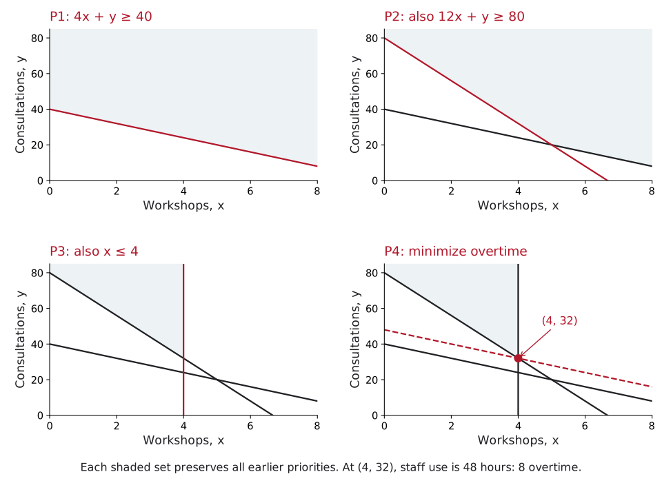
In Solver, implement these priorities as successive solves: minimize the P1 deviation, fix its achieved value, minimize P2, fix that value, and continue. Here the first three achieved values are zero, so the last solve minimizes overtime while keeping those three deviations at zero. Priority labels are an order of solves, not ordinary numeric weights to add in one objective.
The first three goals can all be met together, so each is met in full. The fourth cannot. Four workshops reach 48 clients, the other 32 need consultations, and staff hours come to \(4(4) + 32 = 48\), 8 over. Fewer workshops only make it worse, because each workshop dropped takes 12 consultations to replace, 8 more staff hours net. So the plan is 4 workshops and 32 consultations, with \(d^{-}_{\text{hours}} = d^{-}_{\text{clients}} = d^{+}_{\text{room}} = 0\) and \(d^{+}_{\text{hours}} = 8\). It sits at the corner where the clients line meets the room line. Taylor calls this the most satisfactory solution rather than the optimal one: it meets the goals as well as their order allows, and it says exactly which goal gave way, and by how much.
The order is doing real work. Swap P3 and P4, so the director would rather rent a room than pay overtime, and the same steps land on 5 workshops and 20 consultations: \(60 + 20 = 80\) clients and \(20 + 20 = 40\) staff hours with no overtime, but 10 hours of workshops against the room’s 8, so \(d^{+}_{\text{room}} = 2\) rented hours.
Build the skill 3: when goals tie, weight them instead of ranking them
Preemptive ranking says a higher priority is untouchable: no amount of Priority-4 gain may cost Priority 3 anything, so the director accepts 8 overtime hours to avoid a single rented hour. That is often too rigid. The rented room and the overtime are both costs of the same week, and a director may be willing to trade one against the other. That is non-preemptive, or weighted, goal programming, and it is the other half of Taylor’s treatment.
Put the room overage and the overtime both at Priority 3. Instead of ranking them you attach weights inside the level:
\[P_3\big(2\,d^{+}_{\text{room}} + 1\,d^{+}_{\text{hours}}\big).\]The 2-to-1 ratio says an hour in the rented room across town, off the bus lines that earned Site A its transit score, hurts twice as much as an hour of overtime. Compare the two plans the two orders produced. Four workshops and 32 consultations carry 8 overtime hours, a penalty of \(1 \times 8 = 8\); five workshops and 20 consultations carry 2 rented hours, a penalty of \(2 \times 2 = 4\). Every other plan that keeps P1 and P2 scores worse, so the weighted plan is 5 workshops and 20 consultations. The trade underneath: the fifth workshop takes 2 rented hours and 4 staff hours, and it reaches 12 clients who would otherwise need 12 consultation hours, so it saves \(12 - 4 = 8\) overtime hours, a rate of 4 to 1. Four workshops come back only if the room’s weight is more than 4 times the overtime’s; at exactly 4 the two plans tie, along with every plan on the line between them.
Two things are worth being precise about. The weights trade goals off only within that level. Distinct priority levels stay strictly preemptive, so neither goal may eat into Priority 1 or 2, which is why neither plan buys relief by serving fewer than 80 clients. And the ratio is a judgment, not a measurement. Nothing in the data says a rented hour is twice as bad as an overtime hour; somebody decided that, and a ratio past 4 to 1 returns a different plan.
The practical rule: rank when the goals are genuinely not comparable (the grant’s client target before the room), and weight when they are (a rented room and overtime, two costs you would trade at a stated rate).
In practice: priorities are politics, not just math
- Priorities encode whose goal wins. Ranking the room above overtime puts the clients’ bus routes ahead of the staff’s evenings. The model faithfully executes that choice, but the ranking itself came from people, not data. Of the client target, the room and overtime, whichever the director ranks last is the one that gives way: overtime last gives 4 workshops and 32 consultations (8 hours over), the room last gives 5 and 20 (2 rented hours), and clients last gives 4 and 24 (8 clients short).
- “Most satisfactory” means best under the stated priorities. Goal programming still optimizes: it minimizes unwanted deviations in the specified order, or their weighted sum within a level. Taylor calls the result a most satisfactory solution (satisficing) because conflicting targets may remain unmet. Report the achieved targets and the remaining misses; do not claim that every goal was met or that the model has no mathematical optimum.
- Within-level weights (and the priorities themselves) are judgments too. At 2 to 1 the weighted plan sends a fifth workshop to the rented room; past 4 to 1 it keeps four workshops and pays the 8 overtime hours. Re-run with a few ratios and a few orders, and say where the recommended plan changes.
- The model isn’t the world. Deviation variables assume every miss is equally costly per unit: the eighth overtime hour in a week counts no more than the first, and a client turned away counts the same whether or not they have a hearing next week. Real life has thresholds that a smooth penalty misses. This week’s plans came out in whole numbers; other targets can ask for 4.5 workshops. If half a workshop is impossible, require integer decision variables and solve again; rounding can break a limit or miss the best plan.
Back to the puzzle
The director’s ranking settles the week at 4 workshops and 32 consultations. That meets the first three goals in full: all 40 funded staff hours are used, 48 clients in workshops plus 32 one-on-one make exactly 80, and the workshops fill the community room’s 8 free hours without renting a room. It gives up the fourth goal, overtime, by 8 hours (48 staff hours against 40), and the model says so instead of hiding it. The same numbers under a different order (overtime above the room) or under the 2-to-1 weighting give 5 workshops and 20 consultations: no overtime, and 2 hours in a rented room across town. Goal programming did not choose between those weeks. It let the director’s ranking do the choosing, and it priced what each ranking gives up.
After-class check
Questions spanning weighted scoring and AHP (compute totals, read a pairwise matrix), weight sensitivity, and goal programming (deviation variables, the at-least/at-most → undesired-deviation mapping, and priorities). Retry freely; nothing is submitted.
Weekly take-home (graded: submit on Canvas)
Everything for the take-home goes in one Excel workbook, and it works the same three contractor bids through both of this week’s methods. A city is replacing bus shelters, and one contractor’s safety rating comes from a different auditor on a different scale, so the raw scores cannot be compared until you normalize them. You apply the committee’s weights, test how far the cost weight can move before the ranking flips, and check whether the committee’s AHP pairwise judgments were even consistent enough to use. Then the same bids become a goal program against two published commitments (a spending cap and a minimum number of shelters) and you solve it under both preemptive priority orders, where the answer changes. Two short responses plus the required AI-use disclosure go on the Free responses sheet. Upload the completed .xlsx on Canvas. That one file is your entire submission.