Week 8: Linear Programming: Solver
This week’s big question: real planning problems have dozens of variables and constraints, far too many to draw. How do you solve those? You hand the variables, objective, and constraints to Excel’s Solver, but first you have to understand what makes a plan feasible and what Solver is actually doing.
Before the week
Read: Taylor, Introduction to Management Science (13e), Chapter 3, pp. 97–104. Eight pages, four of them QM for Windows, which this course skips. The chapter PDF is in Canvas Files.
| Pages | Section | This week |
|---|---|---|
| 97–100 | Computer Solution; Excel Spreadsheets | Read. The three cells Solver needs, and what it hands back |
| 100–104 | QM for Windows | Skip, except the passage that opens it (pp. 100–101) on the proper form a constraint must be in, every variable on the left and the constant alone on the right. That is Monday’s standard form; the rest is software this course does not use |
Stop where “Sensitivity Analysis” begins on p. 104. That is Week 9, which reads the second report Solver can print.
Then the warm-up self-check, on an LP’s variables, objective, and constraints:
Session 1: Mon, Oct 12 · From model to spreadsheet
🧩 Puzzle
The tutoring nonprofit. Each week you schedule reading sessions (\(x\)) and math sessions (\(y\)). Each reading session delivers 2 impact points, each math session 3. Room A holds at most 4 reading sessions, Room B at most 5 math sessions, and you have volunteers for at most 7 sessions total. What weekly schedule maximizes impact?
Let \(x\) count reading sessions and \(y\) count math sessions. Maximize their total impact, subject to the room and volunteer limits:
\(\max\ 2x + 3y \quad \text{s.t.}\quad x \le 4,\;\; y \le 5,\;\; x + y \le 7,\;\; x, y \ge 0\).
Build the skill 1: what makes a plan feasible?
Before optimizing, you need to recognize a feasible plan: one that breaks none of the limits. Each constraint divides the plane into “OK” and “not OK”; a plan is feasible only if it is on the right side of every line at once. Drag the dot to try plans and watch which limits turn red:
The set of all feasible plans is the feasible region, the area shaded blue in the widget. Its edges are the two axes and the three limit lines: the reading room at \(x = 4\), the math room at \(y = 5\), and the volunteers at \(x + y = 7\). Every point inside it is a schedule you could actually run, and the dot turns red whenever you drag it outside. For this bounded LP, you can find the best plan at a corner, where two boundary lines meet.
A 10-second feasibility check. You do not need a picture to test a single plan. Just substitute it into every constraint. Is the plan 3 reading, 5 math feasible? Check each limit: reading room \(3 \le 4\) ✓, math room \(5 \le 5\) ✓, volunteers \(3 + 5 = 8 \le 7\) ✗. One violation is enough to make the plan infeasible, because eight sessions need eight volunteers and you only have seven, however good its impact score would have been. This plug-and-check drill is the whole idea behind the dragging widget.
Build the skill 2: the three cells Solver needs
Solver is an Excel add-in. To enable it in desktop Excel, search for Excel Add-ins, open that command, check Solver Add-in (or Solver), and select OK. On a Mac, use the Help search field to find Excel Add-ins. The home page’s Software & setup list has the same instructions.
Illustrated Excel guide: enable Solver with search
These are drawn interface illustrations, using Excel’s command names. Your version’s layout may differ; the setup and cell references are the same.
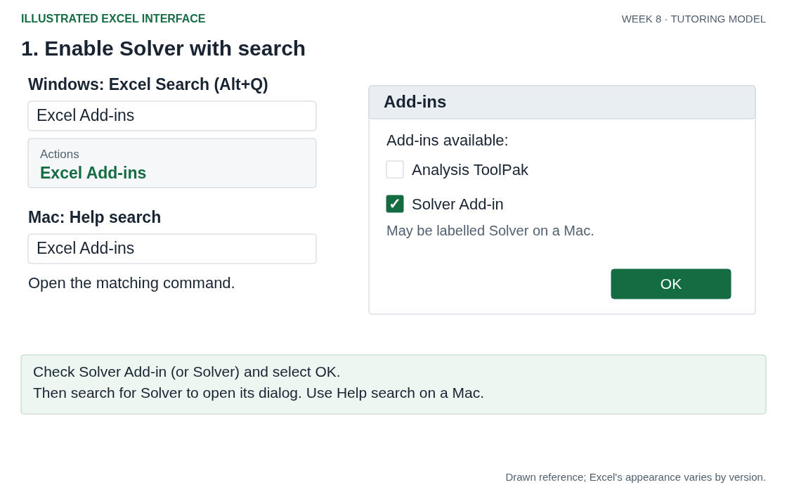
It does for many variables what the graph did for two, but it cannot read a model written in symbols: the LP has to sit in cells, and each of the model’s three ingredients becomes one sort of cell:
| LP part | In Excel |
|---|---|
| decision variables | changing cells: one cell per variable (\(x\), \(y\)), the only cells Solver is allowed to alter |
| objective | objective cell: one formula over the changing cells, =2*x + 3*y, and a direction: maximize |
| constraints | constraint cells: one left-hand-side formula per limit, =x + y, compared to its right-hand side, \(\le 7\) |
Solver chooses the numbers in the changing cells and touches nothing else. The objective cell and the constraint cells are computed from the changing cells, so each time Solver tries a plan they recalculate, and Solver reads them to see how much impact the plan delivers and whether it breaks a limit. Excel’s dialog asks for the same three things in its own words: Set Objective, By Changing Variable Cells (your changing cells), Subject to the Constraints. If you can write the model, you can set up Solver; the skill being assessed is knowing what you asked it to do.
Put it in standard form first. A constraint cell holds everything the plan uses, and the limit beside it is a plain number, so a constraint fits that layout only in standard form: all the variables on the left-hand side, all the constants on the right. Some algebraic methods turn an inequality into an equation by adding a slack variable. Solver needs no slack variable, only this layout, which is what Taylor calls standard form on p. 100. The tutoring model’s three limits are already in it (\(x \le 4\), \(y \le 5\), \(x + y \le 7\)). A rule added to a brief can hide a variable on the wrong side. Three rules the director might add, each as first written and then tidied:
| The rule, as the brief says it | As first written | Standard form |
|---|---|---|
| Spending on math must not exceed spending on reading (a math session costs \$30, a reading session \$25) | \(30y \le 25x\) | \(25x - 30y \ge 0\) |
| Choose a total session count \(z\) as well as its reading/math split | \(x + y = z\) | \(x + y - z = 0\) |
| No more than twice as many reading as math sessions | \(x / y \le 2\) | \(x - 2y \le 0\) |
A variable stranded on the right, like \(z\), or a ratio, like \(x / y\), is the step students trip on most. A ratio is not even linear as written, and it divides by zero in any week with no math sessions. Clear the fraction (\(x \le 2y\), then \(x - 2y \le 0\)) so every constraint is a tidy sum of terms, and do it before you touch the spreadsheet.
Build the skill 3: a worked Solver run (the tutoring model)
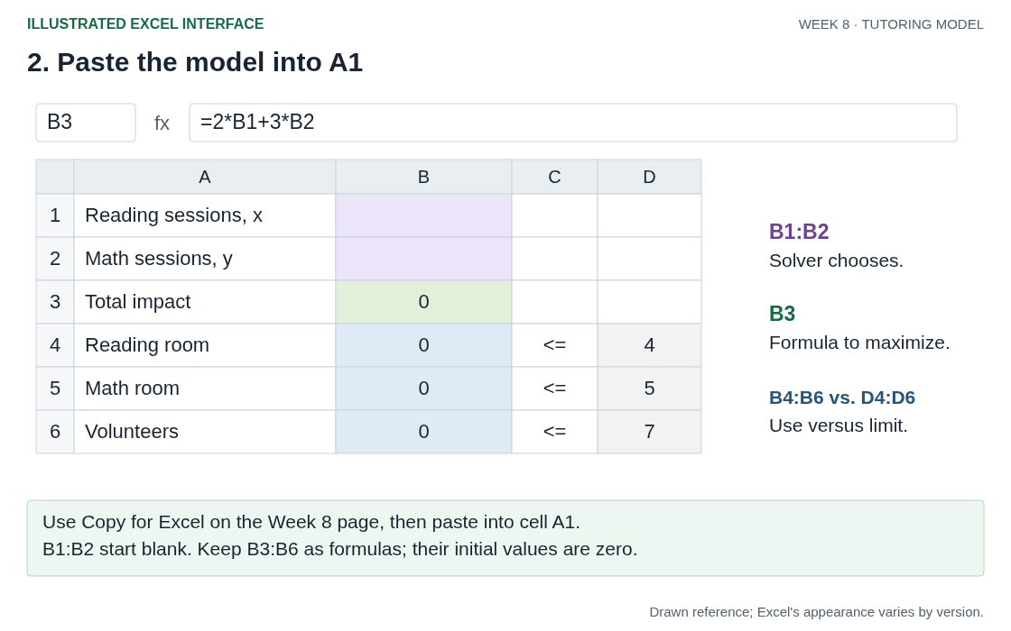
Here is the tutoring model typed into a blank worksheet. In this demonstration, column A holds the labels, column B the cell Solver reads, column C the sign, and column D the limit. The take-home uses its own cell addresses and column headings; match the same three roles to that sheet.
Click Copy for Excel, select cell A1 on a blank worksheet, and paste. The copy includes the six data rows, with formulas and blank changing cells. The row numbers and column letters stay on this page, so the pasted cells match the references below.
| A | B | C | D | |
|---|---|---|---|---|
| 1 | Reading sessions, x | |||
| 2 | Math sessions, y | |||
| 3 | Total impact | =2*B1+3*B2 | ||
| 4 | Reading room | =B1 | <= | 4 |
| 5 | Math room | =B2 | <= | 5 |
| 6 | Volunteers | =B1+B2 | <= | 7 |
- Changing cells, B1 and B2: the only cells Solver may alter. They start empty.
- Objective cell, B3: a formula over B1 and B2, set to Max.
- Constraint cells, B4 to B6: one formula per limit, each held against its limit in column D.
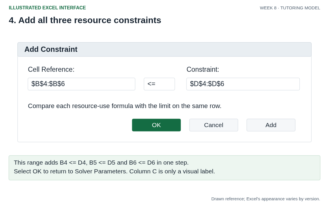
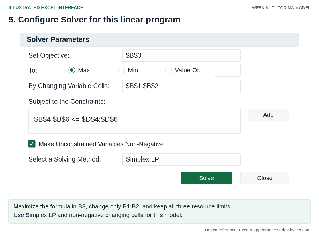
Solver fills two cells, B1 and B2, and the other four are computed from them. That is why B3 through B6 must be formulas that reference B1 and B2, never typed numbers: a 19 typed into B3 stays 19 whatever Solver puts in B1 and B2, so it gives Solver nothing to push up. Search for Solver to open its dialog (use Help search on a Mac). The dialog then reads: Set Objective B3, to Max; By Changing B1:B2; Subject to B4:B6 \(\le\) D4:D6; tick Make Unconstrained Variables Non-Negative for \(x, y \ge 0\); and under Select a Solving Method choose Simplex LP, the method Wednesday opens up. That is the whole setup: two empty cells, one formula to push up, three formulas each held against its limit. Before Solve, verify that changing B1 or B2 changes every formula that depends on it.
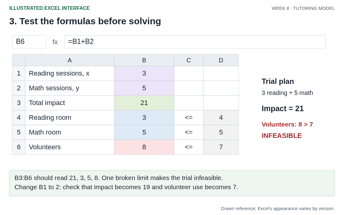
Test the connections before asking Solver to optimize. Temporarily type 3 in B1 and 5 in B2. B3 must change to 21, and B4:B6 to 3, 5, 8. The volunteer row now reads \(8>7\), so this trial is infeasible. Change B1 to 2: the objective becomes 19 and volunteer use becomes 7. If any formula cell stays fixed, repair its references before solving. This check separates a working spreadsheet from numbers merely typed into the right-looking boxes.
Illustrated Excel guide: paste, check, and configure the model
Use the Copy for Excel button above, or open the ungraded tutoring demo workbook. Both put the model in A1:D6. These are drawn interface illustrations; select one to open its full-size picture.
Before you press it, a guess. The illegal week \((3, 5)\) would have scored \(2(3) + 3(5) = 21\). Does Solver’s best legal week beat 21, tie it, or fall short?
Press Solve. 2 and 5 land in B1 and B2: Solver’s pick is 2 reading sessions and 5 math. The objective cell follows: \(2(2) + 3(5) = 19\). The constraint cells read 2, 5 and 7 against 4, 5 and 7: every limit met (\(2 \le 4\), \(5 \le 5\), \(7 \le 7\)), and two rows sit exactly on their limit. So 19 is the most a legal week can score, two short of the illegal 21, because Solver only looks at plans that pass every row. Which rows it ran into is Wednesday’s report.
In practice: a model is only as good as its inputs
- Where do the coefficients come from? “2 impact points per reading session” is an estimate. If it is really a range, your optimum may shift. Wednesday drags it to see how far.
- Whole numbers. Today’s answer came out whole, but nothing in the model asks for that: give the volunteers time for 7.5 sessions and Solver schedules 2.5 reading sessions. If half a session is meaningless, you need integer programming, which Week 10 takes up, not rounding. Rounding 2.5 up to 3 needs 8 sessions of volunteer time against 7.5, and in other models rounding misses the best whole-number plan.
- The four quiet assumptions. Every LP rests on four things being true: proportionality (twice the sessions, twice the impact; no economies of scale), additivity (the total is the sum of the parts, with no interaction between \(x\) and \(y\)), divisibility (fractional values are allowed), and certainty (the coefficients are known, not guessed). If returns diminish, if two activities interfere, or if your numbers are really rough estimates, the model can give a confident-looking answer that is wrong.
Back to the puzzle
The weekly schedule that delivers the most impact is 2 reading sessions and 5 math, for 19 impact points. Solver found it once the brief was a feasible region and three sorts of cell, and the illegal 21 was never on offer; you can tell a legal week from an illegal one yourself in ten seconds by plug-and-check. What you cannot yet say is why that corner and not another, or which limits it ran into. Wednesday answers both: watching Solver walk the region’s corners says why that one, and the report Solver prints names the limits. Writing the limits down correctly stays your job, because Solver only ever searches the plans your constraint cells allow.
In-class group practice (wrap-up)
To close Session 1, formulate a small LP together and map it onto Solver’s three cells.
Write every member’s name on the sheet. You have 15 minutes for the practice, then two minutes to photograph your group’s own attempt before the solutions are shown. One member uploads the photo to Canvas by the end of class; participation credit is for attempting the work.
The instructor uses the final eight minutes to demonstrate the handout’s method, check the main results with units, and explain a common mistake. This demonstration closes the session.
- Download: Week 8 group practice (Word)
Session 2: Wed, Oct 14 · Solver finds the optimum, and explains it
🧩 Puzzle
Monday you wired the tutoring model into Solver, maximize \(2x + 3y\) subject to \(x \le 4\), \(y \le 5\), \(x + y \le 7\), and pressed Solve: 2 reading, 5 math and 19 impact points landed in the cells. A number is not an explanation. A director will ask why that schedule, what is holding it back, and what would change it. How do you know Solver found the best one, and what does it tell you besides the answer?
Build the skill 1: Solver walks the corners
For this bounded, nonempty LP, at least one corner attains the best value. The Simplex LP method searches along edges between corners. Monday’s region has five corners, and you can score every one with \(Z = 2x + 3y\): \((0, 0)\) at 0, \((4, 0)\) at 8, \((4, 3)\) at 17, \((2, 5)\) at 19, and \((0, 5)\) at 15. An illustrative simplex walk visits fewer corners. Start at the origin, \(Z = 0\), where two edges leave: along one, each reading session adds 2 points; along the other, each math session adds 3. It takes the faster climb, math, straight up until the math room is full at \((0, 5)\), where \(Z = 15\). From there the only edge that climbs runs along the top, adding reading sessions at 2 points each, until the volunteers run out at \((2, 5)\), where \(Z = 19\). At \((2, 5)\) both edges lead down, back to \((0, 5)\) at 15 or on to \((4, 3)\) at 17. No neighboring corner scores higher, so it stops: two hops, and it never visits \((4, 0)\) or \((4, 3)\). That improving corner walk illustrates the Simplex Method, the Simplex LP method in the dialog. Excel may take a different route because of its starting basis and preprocessing; the widget shows one valid route. Press Walk corners below and the marker takes the same route, stopping at the origin, at \((0, 5)\) and at \((2, 5)\), and leaves the two edges it travels and each stop’s \(Z\) on the chart. Then press Maximize to slide the objective line out to that same corner. Two views of one fact: the best plan is a corner, and it is that one.
The optimum is 2 reading and 5 math sessions, for 19 impact points. The walk says which corner is best; it does not say which limits are holding the schedule there. The report does.
Build the skill 2: read the Answer Report
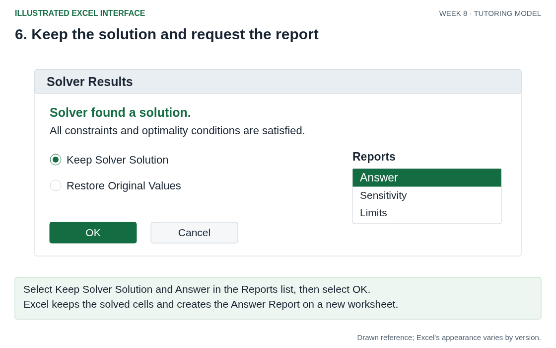
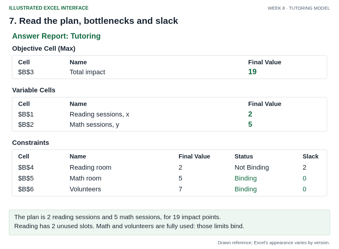
When Solver finishes, choose Keep Solver Solution, select Answer in the Reports list, and select OK. Excel creates the Answer Report on a new worksheet, with a summary in three sections. The Objective (Target) cell section gives the optimal value; the Variable (Adjustable) cells section lists what Solver chose; and the Constraints section reports, for each limit, its Status (Binding or Not Binding) and its Slack. Slack is the leftover (how much of a resource you did not use), so a binding constraint has slack 0 (used to the last unit) and a non-binding one has slack greater than zero. Here is what the report looks like for the tutoring optimum \((x, y) = (2, 5)\):
| Section | Item | Value | Status | Slack |
|---|---|---|---|---|
| Objective cell | total impact | 19 | ||
| Variable cells | reading \(x\) | 2 | ||
| Variable cells | math \(y\) | 5 | ||
| Constraints | reading room \(x \le 4\) | 2 | Not Binding | 2 |
| Constraints | math room \(y \le 5\) | 5 | Binding | 0 |
| Constraints | volunteers \(x+y \le 7\) | 7 | Binding | 0 |
Read it top to bottom: the value, the plan, then each limit’s status and slack (available minus used). You ran 2 of an allowed 4 reading sessions, so the reading room has slack 2 (two unused slots) and is not your limit. The math room and the volunteers are both binding (slack 0): those are your real bottlenecks, and the only two places where more capacity could buy more impact. Renting a bigger reading room buys zero extra impact this week, because two of its four slots already sit empty. Name the binding constraints and the slack on the rest: that sentence is exactly what the graded take-home asks you to read off in Excel, so practice it here first.
Illustrated Excel guide: keep the solution and read the Answer Report
These drawn interface illustrations show the solved tutoring model. Select one to open its full-size picture.
Build the skill 3: what if a coefficient changes?
The impact of a reading session is an estimate. Suppose it rose from 2 to exactly 3. Does the best schedule change, and to what? Drag the impact per reading session slider and watch the optimal corner:
At 3, a tie. The objective is now \(3x + 3y = 3(x + y)\), and every point on the volunteer edge has \(x + y = 7\), so it scores 21 at \((2, 5)\), at \((4, 3)\), and all along the edge between them. When the objective line runs parallel to a binding edge, every point along that edge is optimal. These are multiple optima. Taylor’s heading for the case is multiple optimal solutions, and he calls the two tied corners the alternate optimal solutions. The widget draws the tied edge and names it. Solver does not: its Answer Report prints only the one corner it stopped on, so a tie is yours to spot.
Past 3 it jumps to \((4, 3)\), and at an impact of 4 the line \(4x + 3y = 25\) touches \((4, 3)\) alone. Drag the other way and the plan stays at \((2, 5)\): its two reading sessions run on volunteers the full math room cannot use, so they add impact at any value above 0. Only at exactly 0 does the line lie flat along the math-room edge, where \((0, 5)\) ties: the same case on the other binding edge. The corner never drifts; it stays or it jumps. So “a linear program has exactly one optimal point” is false, and a tie like this is the standard counterexample. How far a coefficient can move before the corner jumps is sensitivity analysis, and it is Week 9’s first question.
A preview of Week 9: what is one more unit of a bottleneck worth? Move a limit instead of a coefficient, on the same region. One more volunteer slot (relax \(x + y \le 7\) to \(\le 8\)): the line moves out one, the corner slides to \((3,5)\), and impact rises from 19 to 21. That one extra slot bought 2 impact points. One more reading slot (\(x \le 5\) instead of \(\le 4\)): the line moves out one, the corner stays at \((2,5)\), and 19 stays 19. Worth 0. That 2 is the volunteer constraint’s shadow price: what one more unit of your bottleneck is worth to the objective. A slack resource is worth nothing more at the margin, which is what the 0 says. Next week’s report prints these for every constraint, and says over what range they hold.
Read the two endpoints and distinguish the two kinds of change
The original plan \((2,5)\) earns \(2c+15\) when a reading session is worth \(c\) impact points. The competing corners \((0,5)\) and \((4,3)\) earn 15 and \(4c+9\). Comparing those totals gives \(0 \le c \le 3\): inside the band the same plan wins, and at either endpoint another corner ties. The objective-line tilt changes which plan is best without moving any resource boundary.
An extra volunteer changes the boundary instead. At 7 volunteer slots the best plan is \((2,5)\) for 19 impact points; at 8 it is \((3,5)\) for 21; at 9 it is \((4,5)\) for 23. Each extra slot in that interval adds 2 impact points. Beyond 9, both rooms are full, so more volunteers add nothing. That is why a shadow price has a range. Week 9 develops the full Sensitivity Report; this is its foundation, and the midterm still draws its questions from the existing Weeks 1–8 self-checks and take-home items.
In practice: read the report, not just the number
- Infeasible or unbounded. For a linear model solved with Simplex LP, “could not find a feasible solution” means no plan satisfies all the entered constraints. “The objective cell values do not converge” means the objective can keep improving without a finite best value. Check the formulas and constraints first: infeasibility can reflect genuinely conflicting requirements, while an unbounded objective often reveals a missing limit.
- Spend effort on what binds. More capacity pays only where the report says binding. Loosening a limit with slack changes nothing until that slack is used up, and other changes can use it up: two more volunteers would move the schedule to \((4, 5)\) and fill the reading room too. Re-read the report after every change.
- The map is not the territory. Solver optimizes your model. If the model omits something real (equity, morale, a soft limit), the “optimal” plan may be a poor decision. Sanity-check the plan against the things the model was never told.
Back to the puzzle
You know 2 reading and 5 math sessions, 19 impact points is the best schedule because the corner walk stopped there: this bounded LP has an optimal corner, and both neighbors of \((2, 5)\) score less, 15 at \((0, 5)\) and 17 at \((4, 3)\). Besides the answer, the Answer Report tells the director what is holding the schedule back: the math room and the volunteers bind, and the reading room has 2 slots to spare. Moving one number at a time says what would change it: the schedule holds until a reading session is worth 3 impact points, and one more volunteer slot adds 2 points while a bigger reading room adds none. Compare the volunteer’s added impact with the cost of getting that help. Solver produces the answer and the report without drawing anything, which is why the same method scales to 200 variables. Solver gives you the answer and the reasons. Read both.
After-class check
Questions spanning feasibility, the Solver setup, standard form, the simplex method, reading the Answer Report, binding constraints and slack, multiple optima, and the four LP assumptions. Retry freely; nothing is submitted.
Weekly take-home (graded: submit on Canvas)
This week’s take-home is an LP solved in Solver for a city public-works department planning a month of street repairs, and when you open the model sheet, nothing on it computes anything. In the Your model block you define the variables and write the objective and all three constraints from the brief, converting a labor pool quoted in worker-days, and name which cells will play Solver’s three roles. You then test one plan by hand, write the objective and constraint cells as live Excel formulas of your own, run Solver, and read its Answer Report to find which limits bind and which one has room to spare. One short recommendation plus the required AI-use disclosure go on the Free responses sheet. Upload the completed .xlsx on Canvas. That one file is your entire submission.
AI use. Tier 1: AI is allowed as a tool here, provided you disclose it on the Free responses sheet and could rebuild and modify the model unaided on an exam. See Using AI.
Audit the AI’s model (optional practice: Tier 2)
A community health clinic asked an AI assistant to build a scheduling LP of its own, a separate case from your graded take-home. It produced a model, ran Solver, and recommended running no flu-shot clinics at all, and its model contains exactly one error. Download the companion workbook, find and fix the flaw, re-solve, and work out what the mistake would have cost the clinic.
Optional and ungraded, but it is excellent preparation for an exam, and the most realistic task in the course: in practice you will inherit someone else’s model far more often than you build one from scratch. AI is allowed and encouraged here (Tier 2. See Using AI).